Intro to Casual Inference
Luis Chancí
lchanci1@binghamton.edu
Econometrics - Econ 466
Department of Economics
Binghamton University
Spring, 2019
Up to Now in Econ 466
Up to Now
Relationship between variables represented by a Linear Model
For instance, summarize the predictive power of schooling’s effect on wages with the conditional expectation function (CEF):
\[\mathbb{E}[log(Salary)_i|X_i]=\beta_0+\beta_1Edu_{i}+\beta_kExper_{i}\]
Up to Now
| Estimate | Std. Error | t value | Pr(>|t|) | |
|---|---|---|---|---|
| (Intercept) | 5.503 | 0.112 | 49.12 | 8.126e-261 |
| educ | 0.07778 | 0.006577 | 11.83 | 3.616e-30 |
| exper | 0.01978 | 0.003303 | 5.988 | 3.022e-09 |
Also
Add some assumptions, and then
- Hypothesis testing
- ``Casual effect" (?)
After midterm 1, some assumptions may fail, for instance,
- Heteroskedasticity
- Serial correlation
Endogeneity
One relevant part we reviewed was:
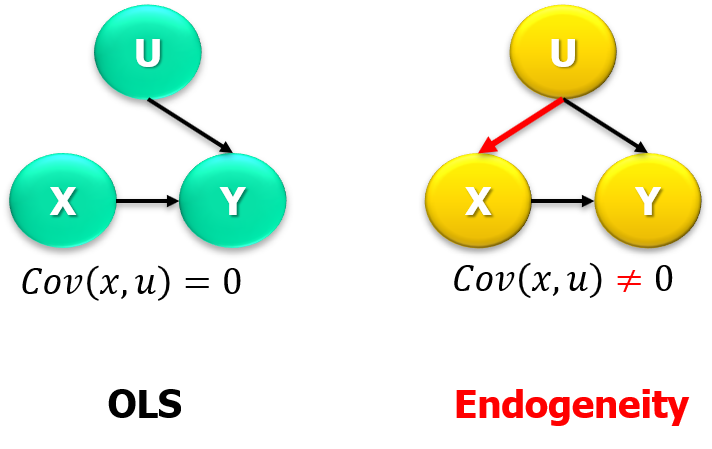
Endogeneity
- Recall Omitted Variable Bias,
\[\begin{eqnarray} \mathbb{E}(\hat{\beta}_{1}|X)\equiv\beta_1+\beta_2\frac{Cov(X,Omitted\,Part)}{Var(X)} \end{eqnarray}\]
- Because of endogeneity, the causal effect cannot be identified.
Causality
Again: Correlation and Causation
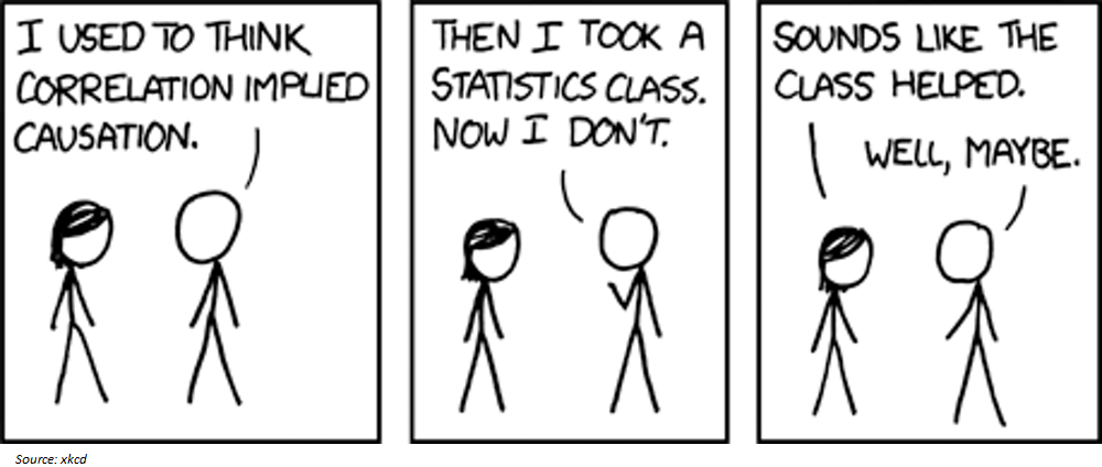
(there are many correlations that are not causal)
Causal Effect
How do we know if \(X\) causes \(Y\)?
E.g., causal relationships
- Light switch turned on => light to be on
- College degree => earnings (?)
Discussion
- what causality is and how we can find it
- research designs for uncovering causality
Causal Effect
Causal Effect
Pick up one observation: \(i=Luis\)
Crazy idea, assume there are two parallel universes (PU):
- In PU1: Luis has a college degree, \(X_i^0\), then observe earnings, \(Y_i^0\).
- In PU2: (same) Luis has a Ph.D., \(X_i^1\), then observe earnings, \(Y_i^1\).
EVERYTHING is the same, EXCEPT Schooling.
Hence, we can conclude with respect to differences in earnings.
Causal Effect
In practice there is one issue,
a prediction of what would have happened in the absence of the treatment.
Causal Inference
Outline
Notions: Treatment, Control, Experiment, Quasi-Experiment, others.
Methods:
- Selection on unobservables
- Differences-in-differences
- Panel methods
- Instrumental Variables
- Selection on observables:
- Regression
- Regression Discontinuity Design
- Matching
Treatment and Control
Let’s use a dummy variable for whether an observation, \(i\), received a treatment or not:
Treatment: \(D_i=1\)
Control: \(D_i=0\)
There is an ACTUAL outcome: \(Y_i\)
and an UNOBSERVED counterfactual:
\[ Unobserved\,outcome= \left\{ \begin{array}{c} Y_i^1&if&D_i=1\\ Y^0_i&if &D_i=0 \end{array} \right. \]
Experiments
Experiments
We would like to compare two observations that are basically exactly the same except that one has \(D=0\) and one has \(D=1\).
Experiments:
- research design (control the assignment to treatment)
- direct manipulation of subjects’ values on \(X\)
- measure changes in the values on \(Y\)
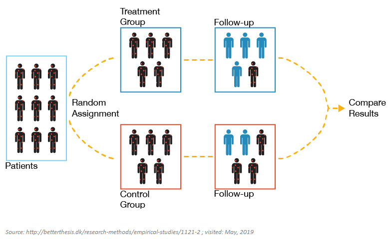
Randomized Controlled Trial, RCT
Experiments
Experiments
The econometric specification could be as simple as,
\[Y_i=\beta_0+\beta_1D_i+u_i\] which is the same as a two-sample t-test.
\(\,\)
On the other hand, there are some challenges to consider. For instance,
- Practical issues (e.g., randomizing types of exchange rate systems for developing countries).
- Ethical issues.
- “Too” controlled.
Natural Experiments
- The control and experimental variables of interest are not artificially manipulated by researchers
- Nature does the randomization
- Exogenous source of variation that determine treatment assignment
- Examples:
- policy changes
- government randomization
Quasi-experiments
Experiments and Quasi-experiments:
In an experiment, participants are randomly assigned to treatment or control.
In a quasi-experiment, observations are not assigned randomly.
Thus,
Groups may differ not only in treatment
(need to statistically control for differences).
There may be several “rival hypotheses” competing with the experimental manipulation as explanations for observed results.
Methods
Some Standard Methods
- Fixed effects
- Differences-in-Differences
- Instrumental Variables
- Regression Discontinuity
Fixed Effects
Fixed Effects
Idea,
- Again, recall Omitted Variable Bias
- We cannot control for many things
- measurement issues
- data issues
\(\,\)
- But, if we observe each observation \(i\) multiple times \(t\),
- control for each observation identity.
- it would be like “trying to control for everything unique” to that observation.
Panel Data
library(foreign)
Panel <- read.dta("http://dss.princeton.edu/training/Panel101.dta") # Source: http://dss.princeton.edu/training, visited Apr 2019.| country | year | y | y_bin | x1 | x2 | x3 | opinion |
|---|---|---|---|---|---|---|---|
| A | 1990 | 1342787840 | 1 | 0.2779036 | -1.1079559 | 0.2825536 | Str agree |
| A | 1991 | -1899660544 | 0 | 0.3206847 | -0.9487200 | 0.4925385 | Disag |
| A | 1992 | -11234363 | 0 | 0.3634657 | -0.7894840 | 0.7025234 | Disag |
| A | 1993 | 2645775360 | 1 | 0.2461440 | -0.8855330 | -0.0943909 | Disag |
| A | 1994 | 3008334848 | 1 | 0.4246230 | -0.7297683 | 0.9461306 | Disag |
| A | 1995 | 3229574144 | 1 | 0.4772141 | -0.7232460 | 1.0296804 | Str agree |
| A | 1996 | 2756754176 | 1 | 0.4998050 | -0.7815716 | 1.0922881 | Disag |
| A | 1997 | 2771810560 | 1 | 0.0516284 | -0.7048455 | 1.4159008 | Str agree |
| A | 1998 | 3397338880 | 1 | 0.3664108 | -0.6983712 | 1.5487227 | Disag |
| A | 1999 | 39770336 | 1 | 0.3958425 | -0.6431540 | 1.7941980 | Str disag |
| B | 1990 | -5934699520 | 0 | -0.0818500 | 1.4251202 | 0.0234281 | Agree |
| B | 1991 | -711623744 | 0 | 0.1061600 | 1.6496018 | 0.2603625 | Str agree |
| B | 1992 | -1933116160 | 0 | 0.3537852 | 1.5937191 | -0.2343988 | Agree |
| B | 1993 | 3072741632 | 1 | 0.7267770 | 1.6917576 | 0.2562243 | Str disag |
| B | 1994 | 3768078848 | 1 | 0.7193949 | 1.7414261 | 0.4117495 | Disag |
| B | 1995 | 2837581312 | 1 | 0.6715466 | 1.7083139 | 0.5358430 | Str disag |
| B | 1996 | 577199360 | 1 | 0.8198573 | 1.5324961 | -0.4996490 | Str agree |
| B | 1997 | 1786851584 | 1 | 0.8801672 | 1.5021962 | -0.5762677 | Disag |
| B | 1998 | -149072048 | 0 | 0.7045161 | 1.4236463 | -0.4484192 | Agree |
| B | 1999 | -1174480128 | 0 | 0.2369673 | 1.4545859 | -0.0493640 | Str disag |
Exploring Panel Data
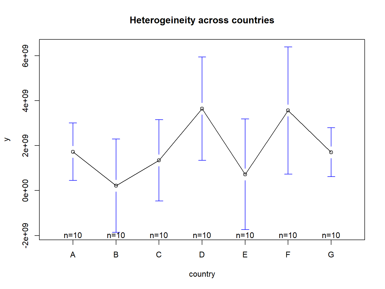
Exploring Panel Data
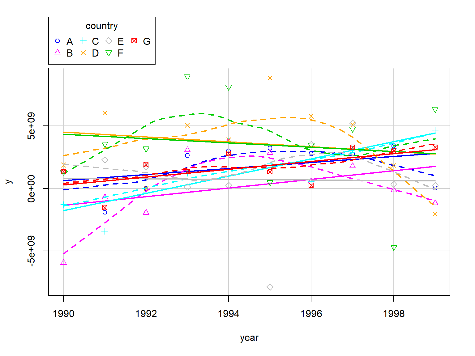
Fixed Effects
For instance, the model could be like
\[\begin{eqnarray} y_{it}&=&\beta_0+\beta_1x_{it}+\underbrace{\boldsymbol{\theta}_{i}}_{FE}+u_{it} \end{eqnarray}\]
\(\,\)
where, \(\theta\) could represent (unobserved) characteristic(s)
Fixed Effects
If we ignore \(\theta_i\),
| Estimate | Std. Error | t value | Pr(>|t|) | |
|---|---|---|---|---|
| (Intercept) | 1.524e+09 | 621072624 | 2.454 | 0.01668 |
| x1 | 4.95e+08 | 778861261 | 0.6355 | 0.5272 |
(not stat. significant)
Fixed Effects
F.E. Estimation
Dummy variable regression, \[y_{it}=\alpha_AD_A+\alpha_BD_B+...+\beta_1x_{it}+u_{it}\] \(\,\)
Within Estimator, \[(y_{it}-\bar{y}_i)\,\,on\,\,(x_{it}-\bar{x}_i)\]
\(\,\)
- First Differencing, \[(y_{it}-y_{it-1})\,\,on\,\,(x_{it}-x_{it-1})\]
Fixed Effects
Dummy Variable Regression,
| Estimate | Std. Error | t value | Pr(>|t|) | |
|---|---|---|---|---|
| x1 | 2.476e+09 | 1.107e+09 | 2.237 | 0.02889 |
| factor(country)A | 880542404 | 961807052 | 0.9155 | 0.3635 |
| factor(country)B | -1.058e+09 | 1.051e+09 | -1.006 | 0.3181 |
| factor(country)C | -1.723e+09 | 1.632e+09 | -1.056 | 0.2951 |
| factor(country)D | 3.163e+09 | 909459150 | 3.478 | 0.0009303 |
| factor(country)E | -602622000 | 1.064e+09 | -0.5662 | 0.5733 |
| factor(country)F | 2.011e+09 | 1.123e+09 | 1.791 | 0.07821 |
| factor(country)G | -984717493 | 1.493e+09 | -0.6597 | 0.5119 |
(stat. significant)
Fixed Effects
Dummy Variable Regression, 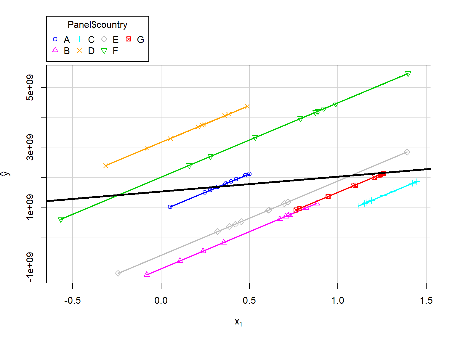
Fixed Effects
Within Estimator,
\[(y_{it}-\bar{y}_i)=\beta_1(x_{it}-\bar{x}_i)+\epsilon_{it}\]
library(plm)
FE <- plm(y ~ x1, data=Panel, index=c("country", "year"), model="within")
pander(coefficients(summary(FE)))| Estimate | Std. Error | t-value | Pr(>|t|) | |
|---|---|---|---|---|
| x1 | 2.476e+09 | 1.107e+09 | 2.237 | 0.02889 |
(stat. significant)
Fixed Effects
Discussion (from Wooldridge)
Strict exogeneity in the original model has to be assumed
In the case T = 2, fixed effects and first differencing are identical
For T > 2, fixed effects is more efficient if classical assumptions hold
If T is very large (and N not so large), the panel has a pronounced time series character and problems such as strong dependence arise
First differencing may be better in the case of severe serial correlation in the errors
Differences-in-Differences
Differences-in-Differences
Motivation
 Doctor John Snow, physician. London, 1813-1858.
Cholera,
- in the early 1800s
- three main waves
Jhon noticed variations
- water supply
- rates of cholera
Differences-in-Differences
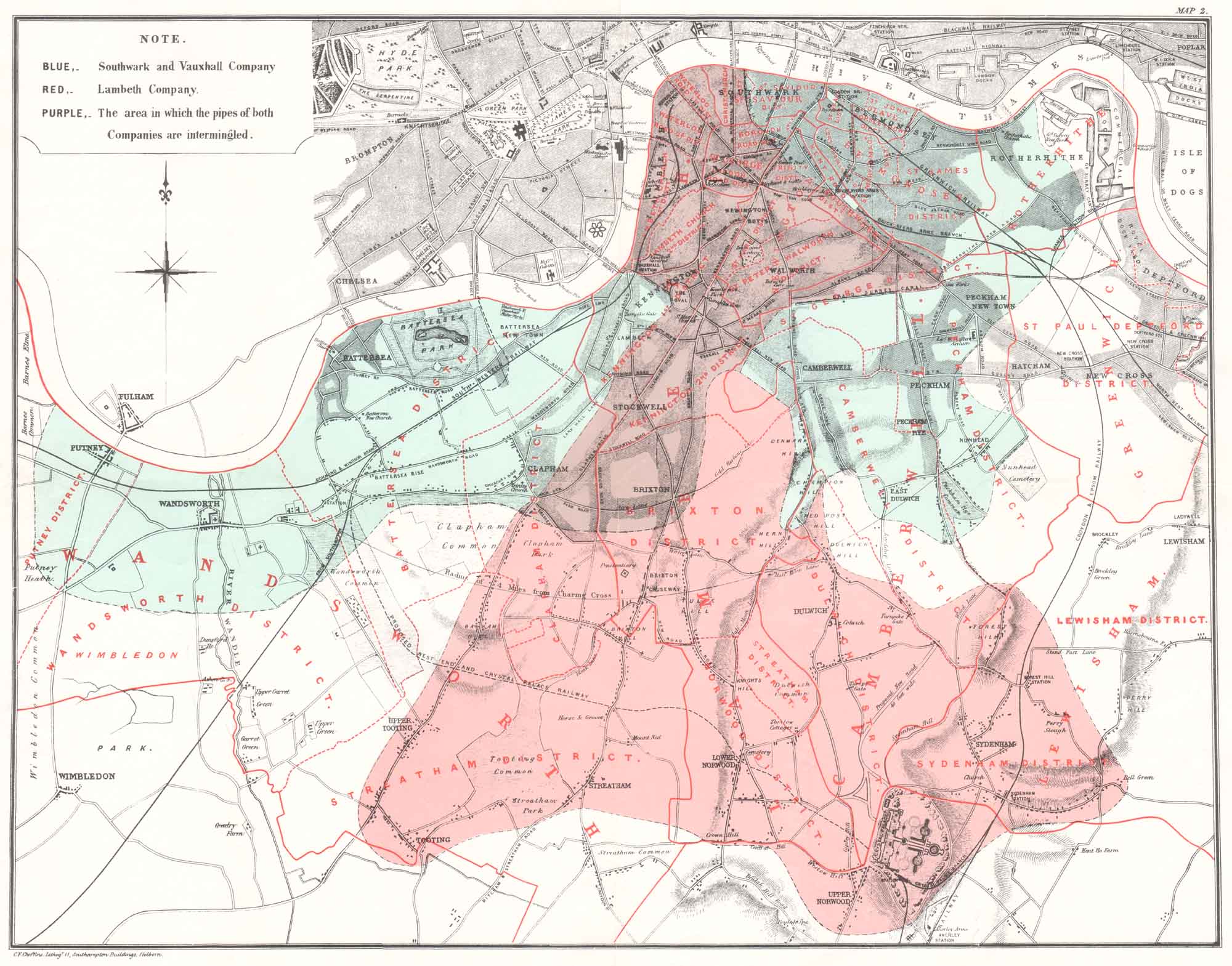
Differences-in-Differences
1849:
- London’s worst cholera epidemic
- Two main companies supplied water:
- Lambeth Waterworks Co.
- Southwark and Vauxhall Water Co
1852: Lambeth Waterworks moved their intake upriver
1853: London has another cholera outbreak
Differences-in-Differences
Do you want to learn more?
Differences-in-Differences
Illustration, 
Differences-in-Differences
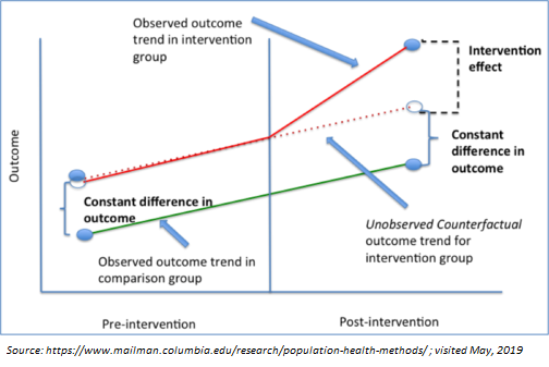
Differences-in-Differences
Econometric specification,
\[y=\beta_0+\beta_1D_{treatment}+\beta_2D_{post}+\beta_3(D_{treatment}*D_{post})+u\]
\(\beta_3\) is the parameter of interest.
Notices that this is related to FE. For instance, if we have more than two groups (T/C = g) and more than two periods (Pre/Post = t):
\[y_{igt}=\beta_0+\beta_1D_{g}+\beta_2D_{t}+\beta_3D_{gt}+\beta_4X_{igt}+u_{igt}\]
Differences-in-Differences
Key Assumptions:
Time affected the Treatment and Control groups equally
Differences-in-Differences
Do you want to learn more?
Instrumental Variables
Instrumental Variables
Idea,
For the linear model, \(y=\beta_0+\beta_1x+u\),
say that we do not have random assignment
but, what if we can find another variable \(z\) with random assignment that causes \(X\)
if this is the case, we coud get a natural experiment!
This variable is called it an “instrument” or “instrumental variable”
Instrumental Variables
Conditions for instrumental variable:
- Does not appear in regression equation
- Is uncorrelated with error term
- Is partially correlated with endogenous explanatory variable
Instrumental Variables
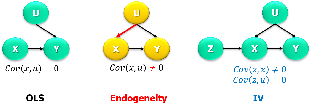
In other words,
There is an endogeneity issue, \[Cov(x,u)\neq 0\]
but, what if we can find \(z\), such as this variable
- causes \(x\) (relevance):
\[Cov(z,x)\neq 0\]
- is randomly assigned, and the only relationship with \(y\) is through \(x\) (exogeneity):
\[Cov(z,u)= 0\]
Instrumental Variables
Instrumental Variables
Before moving on, check
Instrumental Variables
Estimation for \(k=2\), \(y=\alpha+\beta x+u\).
\[If\,\,\,\,Cov(z,u)=0,\,\,\Rightarrow\,\,Cov(z,y)-\beta Cov(z,x)=0\]
thus,
\[\hat{\beta}_{IV} = \frac{\sum{(z_i-\bar{z})(y_i-\bar{y})}}{\sum{(z_i-\bar{z})(x_i-\bar{x})}}\]
Cigarette smoking and child birth weight.
| Estimate | Std. Error | t value | Pr(>|t|) | |
|---|---|---|---|---|
| (Intercept) | 4.769 | 0.005369 | 888.3 | 0 |
| packs | -0.08981 | 0.01698 | -5.29 | 1.422e-07 |
| Estimate | Std. Error | t value | Pr(>|t|) | |
|---|---|---|---|---|
| (Intercept) | 4.448 | 0.9082 | 4.898 | 1.082e-06 |
| packs | 2.989 | 8.699 | 0.3436 | 0.7312 |
Instrumental Variables
Properties of IV with a poor instrumental variable (for \(k=2\)),
\[\begin{eqnarray} plim\,\hat{\beta}_{OLS}&=&\beta_1+Corr(x,u)\frac{\sigma_u}{\sigma_x}\\ & &\\ plim\,\hat{\beta}_{IV}&=&\beta_1+\frac{Corr(z,u)}{Corr(z,x)}\frac{\sigma_u}{\sigma_x} \end{eqnarray}\]
IV worse than OLS if \(\frac{Corr(z,u)}{Corr(z,x)}>Corr(x,u)\)
Instrumental Variables
IV estimation in the multiple regression model (\(k>2\)),
\[y=\beta_0+\beta_1\underbrace{x_{1}}_{Endog}+\beta_2\underbrace{x_{2}}_{Exog}+u\]
Two Stage Least Squares (2SLS)
Stage one (reduced form):
Estimate, \(x_1=\gamma_0+\gamma_1z+\gamma_2x_2+\epsilon\) , to get \(\hat{x}_1\)
Stage two:
Estimate, \(y=\beta_0+\beta_1\hat{x}_{1}+\beta_2x_{2}+u\)
Card(1995), College Proximity as an IV for Education (Example 15.4)
data("card")
reg.ls  <-lm   (lwage~educ   + exper+expersq+black+smsa+south+smsa66+reg662+reg663+reg664+reg665+reg666+reg667+reg668+reg669, data = card)
reg.iv  <-ivreg(lwage~educ   + exper+expersq+black+smsa+south+smsa66+reg662+reg663+reg664+reg665+reg666+reg667+reg668+reg669|
nearc4 + exper+expersq+black+smsa+south+smsa66+reg662+reg663+reg664+reg665+reg666+reg667+reg668+reg669, data = card)| lwage | ||
| OLS | IV | |
| educ | 0.075*** | 0.132** |
| (0.003) | (0.055) | |
| exper | 0.085*** | 0.108*** |
| (0.007) | (0.024) | |
| expersq | -0.002*** | -0.002*** |
| (0.0003) | (0.0003) | |
| Observations | 3,010 | 3,010 |
| Note: | p<0.1; p<0.05; p<0.01 | |
Instrumental Variables
Testing for endogeneity of \(x_1\) in
\[y=\beta_0+\beta_1x_1+\beta_2x_2+u\]
Reduced form, \(x_1=\gamma_0+\gamma_1z+\gamma_2x_2+\epsilon\)
\(x_1\) is exogenous if and only if \(\epsilon\) is correlated with \(u\)
Test equation
\[y=\beta_0+\beta_1x_1+\beta_2x_2+\delta\hat{\epsilon}+e\]
\(H_0\), \(exogeneity\) of \(x_1\), is rejected if \(\delta\) is significantly different from zero.
Regression Discontinuity Design
Regression Discontinuity Design
Motivating Examples
- National Merit Scholarship and GPA.
- Endogeneity issue:
- students performing well => more likely to win
- and continue performing well
- thus, it’s not clear the causal effect of the schoolarship on GPA
- Endogeneity issue:
- Class size and Students reading achievement (Angrist and Lavy, 1997).
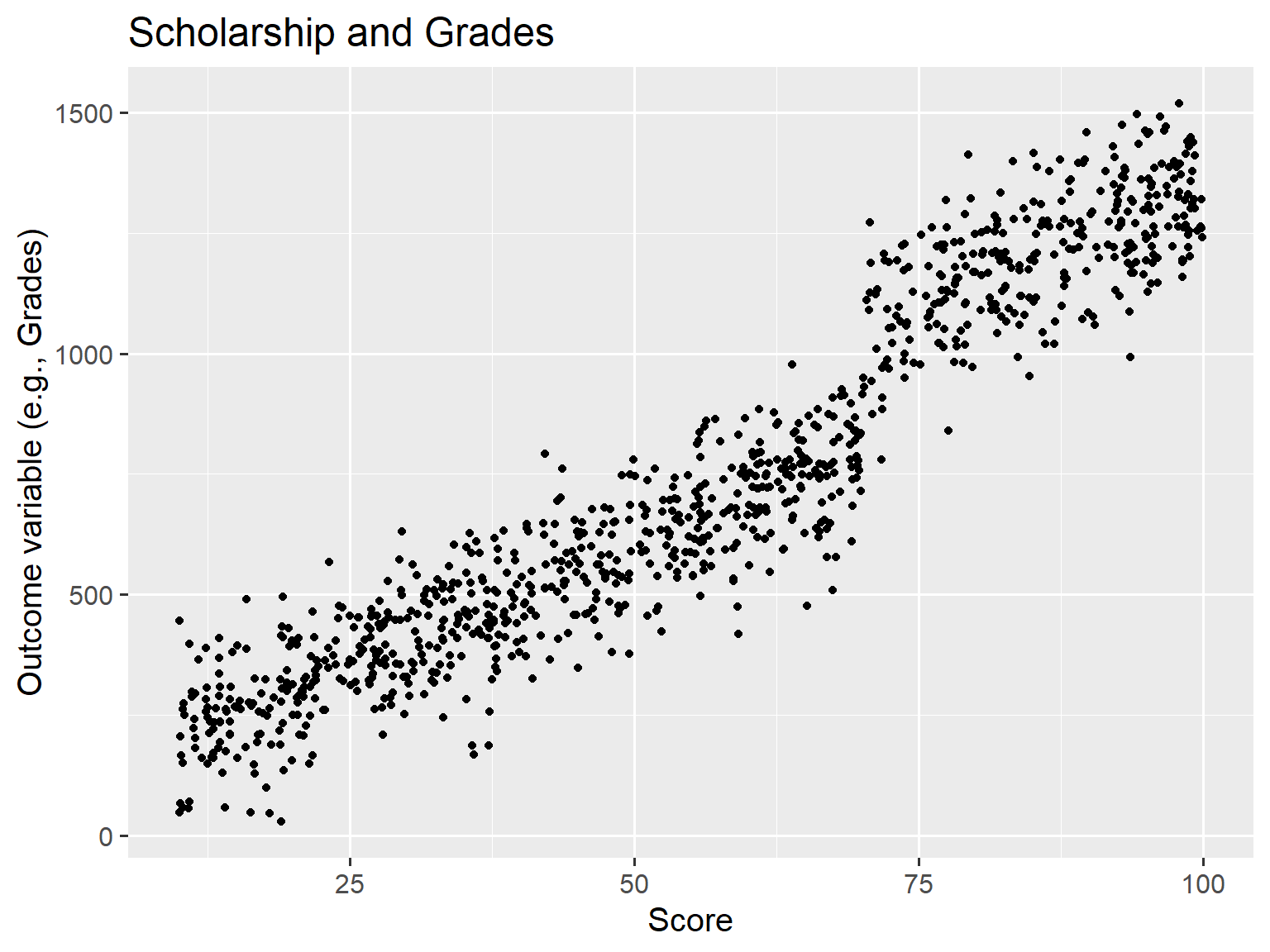
Regression Discontinuity Design - basic idea
RDD exploits exogeneity in program characteristics (designing aspects).
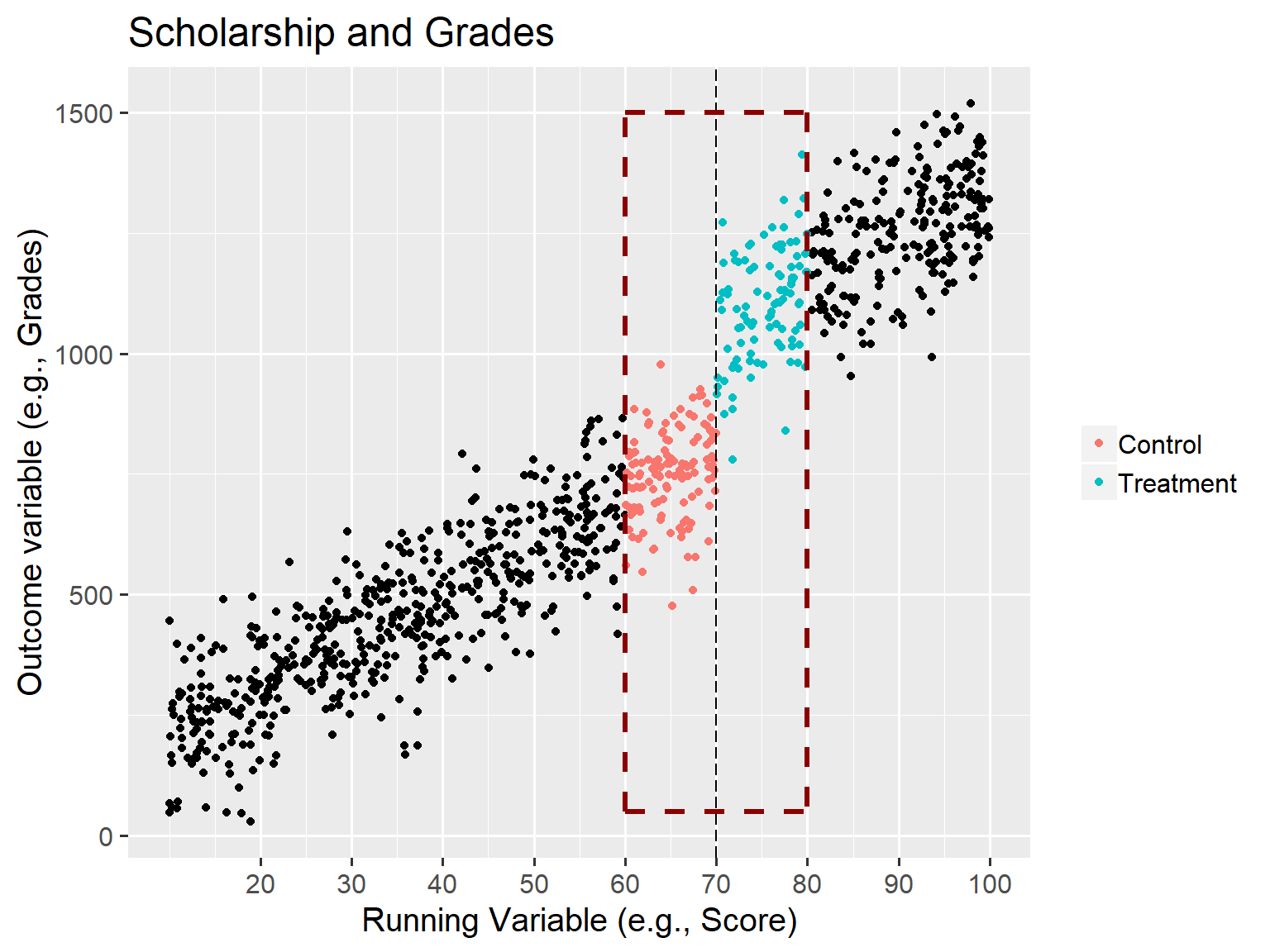
We could think of it as a randomized experiment at cutoff \ Treatment is assigned based on a cutoff (or running variable).
Intuition: Participants in the program are very different, however, at the margin (cutoff), those just at the threshold are virtually identical.
Regression Discontinuity Design - basic idea
For instance,
- scholarship allocation based on scoring above a certain threshold on the PSAT.
- being admitted to a training program based on a test score.
- class size design using Maimonides’ rule.
RDD - Scholarship and Grades
RDD - Scholarship and Grades (2)
RDD - General Idea
(Animation) Source: Nick C. Huntington-Klein. Twitter @nickchk
Ather example. Alcohol and Mortality (Before 1984, MLDA<21)
library(foreign); library(ggplot2)
RDData <- read.dta("http://masteringmetrics.com/wp-content/uploads/2015/01/AEJfigs.dta"); RDData$over21 <- (RDData$agecell>=21); attach(RDData);
ggplot(RDData,aes(x=agecell, y=all,colour=over21))+geom_point()+ylim(80,110)+stat_smooth(method=loess)+labs(x="Age",y="Mortality Rate (per 100,000)") 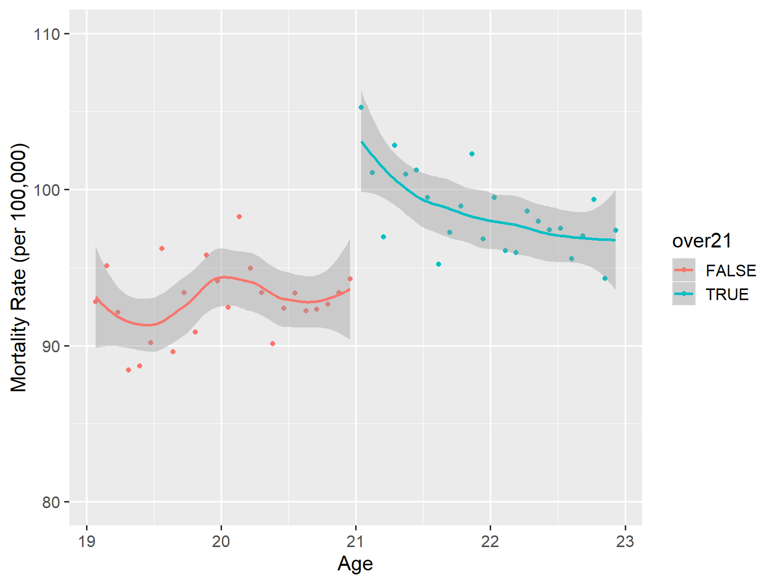
Regression Discontinuity Design
Model
\[y=\beta_0+\beta_1D_{treatment}+\beta_2Running+u\]
Final comments,
- Sharp RDD
- Fuzzy RDD
- Functional form specification
- External / Internal Validity