Ordinary Least Squares (OLS)
Magíster en Economía
Teoría Econométrica (Econometric Theory)
Outline
- Preliminaries: Conditional Modeling - The CEF and regression fundamentals
- The Linear Regression Model (LRM) - Objective function and normal equations
- Geometry and FWL Theorem - Projection matrices and “partialling out”
- Finite-Sample Properties - Unbiasedness, Variance, and Gauss-Markov
- Constrained Least Squares (CLS) - Imposing linear restrictions
- Inference in OLS - Exact distributions and \(t\)/\(F\) tests
- OLS and Gaussian Quasi-MLE - A brief overview of a topic to be discussed later.
- Information Criteria (AIC and BIC) - Model Selection.
- Prediction and Forecast
References
These slides closely follow the lecture notes I prepared for OLS, which are primarily based on:
- Hansen, B. (2022). Econometrics. Princeton University Press.
- Davidson, R., & MacKinnon, J. G. (2004). Econometric Theory and Methods. Oxford University Press.
Our goal is to look “under the hood” of OLS. We will separate the algebraic requirements needed to compute estimates from the statistical assumptions required for inference.
1. Regression as Conditional Modeling
Conditional Expectation Function (CEF)
Let the data be denoted by \(\{w_i\}_{i=1}^N\), where \[ w_i=(y_i,x_i), \qquad y_i\in\mathbb{R}, \qquad x_i\in\mathbb{R}^k. \]
The joint density can always be factored into a conditional and a marginal component: \[ f(y_i,x_i;\theta)=f(y_i\mid x_i;\theta_1)\cdot f(x_i;\theta_2). \]
When we talk about regression, our main object of interest is the conditional component, \[ f(y_i\mid x_i;\theta_1). \]
That is, regression seeks to characterize how the distribution of the outcome \(y\) systematically varies with the covariates \(x\).
Conditional Expectation Function (CEF)
Rather than modeling the full conditional density, we can focus on one of its moments.
The natural starting point is the conditional mean. In particular, the Conditional Expectation Function (CEF) is defined as \[ m(x_i)\equiv \mathbb{E}[y_i\mid x_i]. \]
This object plays a central role in econometrics because it summarizes how the average value of the outcome changes with the covariates.
Much of econometrics can be viewed as (i) estimating the CEF, or some feature of it, and (ii) asking what additional structure is needed to give that object a causal interpretation.
The Linear CEF
Now define the regression error as the deviation from the conditional mean: \[ u_i\equiv y_i-m(x_i) \qquad \Longrightarrow \qquad y_i=m(x_i)+u_i. \]
Important: This decomposition is a definition, not an assumption. By construction, \(\mathbb{E}[u_i\mid x_i]=0\).
A leading special case arises when the CEF is linear: \(m(x_i)=x_i'\beta\).
This gives the Linear Regression Model: \[ y_i=x_i'\beta+u_i, \qquad \mathbb{E}[u_i\mid x_i]=0. \]
Orthogonality and Its Implications
Because \(\mathbb{E}[u_i\mid x_i]=0\), the Law of Iterated Expectations implies \[ \mathbb{E}[u_i]=0. \]
More generally, we obtain unconditional orthogonality: \[ \mathbb{E}[h(x_i)u_i]=0 \qquad \text{for any measurable } h(\cdot), \] and in particular, \(\mathbb{E}[x_i u_i]=0\).
This orthogonality condition is the foundation of moment-based estimation.
If orthogonality fails, for example because of endogeneity arising from omitted variables, simultaneity, or measurement error, OLS will typically converge to the wrong object. Other estimators, such as IV and GMM, are designed for this case.
Statistical vs. Structural Models
Statistical Models. Up to this point, everything has been a statistical statement. The decomposition \(y_i=m(x_i)+u_i\) describes conditional averages in the observable data, but it does not by itself have causal content.
Structural Models are motivated by economic theory and are intended to represent behavioral, technological, or institutional relationships. This is where identification becomes central.
- If a parameter is identified, then in principle it can be recovered from the observable distribution.
- If it is not identified, then more data alone will not solve the problem; additional assumptions or structure are needed.
- The empirical question is not only how to estimate \(\beta\), but also whether the object being estimated has the interpretation we want to give it.
2. The Linear Regression Model
Linearity
A natural and highly tractable way to model the Conditional Expectation Function is to approximate it with a linear function. This leads to the Linear Regression Model.
Assumption 1 — Linearity
\[y_i = x_i'\beta + u_i,\qquad i=1,\ldots,N\]
In matrix form, stacking all \(N\) observations: \[y = X\beta + u\]
where \(y \in \mathbb{R}^{N\times 1}\), \(X \in \mathbb{R}^{N\times k}\), \(\beta \in \mathbb{R}^{k\times 1}\), \(u \in \mathbb{R}^{N\times 1}\).
This linear representation is the starting point for the algebra of OLS and for the finite-sample and asymptotic results that follow later.
Linearity
Interpretation of \(\beta_j\) (semi or elasticity)
The coefficient \(\beta_j\) is usually interpreted as a ceteris paribus effect.
- The interpretation depends on the functional form of the model:
| Model | Dependent variable | Regressor | Interpretation |
|---|---|---|---|
| Level–level | \(y\) | \(x\) | \(\Delta y = \beta_j\,\Delta x\) |
| Log–level | \(\log(y)\) | \(x\) | \(\%\Delta y \approx 100\beta_j\,\Delta x\) |
| Log–log | \(\log(y)\) | \(\log(x)\) | \(\%\Delta y = \beta_j\,\%\Delta x\) |
Interpretation of \(\beta_j\) (Dummy variables)
- Interpretation also depends on the nature of the regressor. If \(x_j\) is a dummy variable, \(\beta_j\) measures the difference in the conditional mean between the group for which the condition holds.
For example, if \(x_j\) is used to indicate race, gender, or treatment status, then \(\beta_j\) captures the corresponding conditional differential relative to the baseline category. - This may change if there are qualitative regressor variables (dummies) - in levels or interactions,
\[D_i= \left\{ \begin{array}{ccl} 1&\text{if}&\text{Condition is met}\\ 0&\text{if}&\text{Condition is not met}\\ \end{array} \right. \hspace{0.6cm} \Rightarrow \hspace{0.6cm} Y_i = \beta_1 + \beta_2 D_i + \beta_3 X_i+\beta_4 (D_i\cdot X_i) + u_i\]
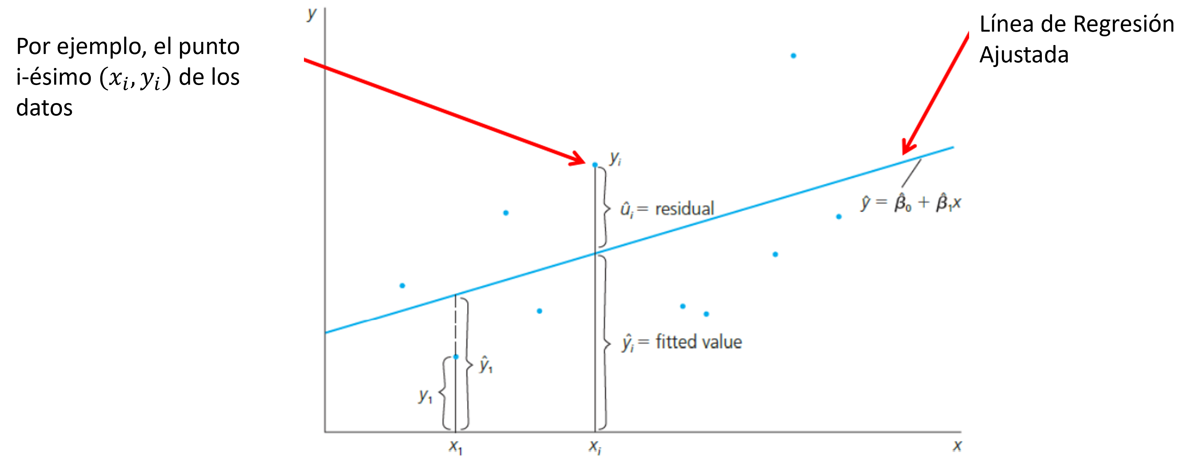
The OLS Objective Function
For observation \(i\), the model error is \(u_i = y_i - x_i'\beta\). After estimation, the sample analog, \(\hat u_i = y_i - x_i'\hat\beta\) is called the residual.
To estimate \(\beta\), Ordinary Least Squares (OLS) chooses the parameter vector that minimizes the sum of squared residuals: \[ \hat{\beta} = \arg\min_{\beta} S(\beta), \qquad S(\beta) = (y-X\beta)'(y-X\beta). \]
The logic is straightforward: squaring the residuals penalizes large errors and treats positive and negative deviations symmetrically.
Expanding the objective function gives \(S(\beta)=y'y-2\beta'X'y+\beta'X'X\beta\).
The FOC
Taking derivatives with respect to \(\beta\) and setting them equal to zero yields the first-order condition: \[ \left.\frac{\partial S(\beta)}{\partial\beta}\right|_{\beta=\hat\beta} = -2X'y+2X'X\hat\beta=0. \]
This first-order condition is the key step that leads to the normal equations.
Rearranging the first-order condition gives the fundamental normal equations: \[X'X\hat\beta = X'y\]
But, to solve this system for a unique \(\hat\beta\), we need an invertibility condition.
The OLS Estimator
Assumption 2 — Full Rank
The regressor matrix \(X \in \mathbb{R}^{N\times k}\) satisfies \(\operatorname{rank}(X)=k\). Equivalently, there is no exact multicollinearity among the regressors.
Under Assumption 2, the matrix \(X'X\) is symmetric positive definite and therefore invertible. Hence, \[ \boxed{\hat\beta_{\text{OLS}}=(X'X)^{-1}X'y.} \]
Two immediate implications are worth keeping in mind. (i) The second-order condition is \(\frac{\partial^2 S(\beta)}{\partial\beta\,\partial\beta'}=2X'X \succ 0\), so the OLS solution is the unique global minimum. (ii) The normal equations also imply \(X'\hat u = X'(y-X\hat\beta)=0\), which means that the residual vector is orthogonal to every column of the regressor matrix.
3. Geometry and FWL Theorem
Projection Matrices \(P\) and \(M\)
Once the OLS estimator has been obtained, the fitted values and residuals admit a useful geometric interpretation. The fitted values (\(\hat{y}= X\hat\beta\)) and residuals (\(\hat{u}=y-\hat{y}\)) can be written compactly using two matrices:
- Projection Matrix (\(P\)): Maps \(y\) onto the column space of \(X\), \(\operatorname{col}(X)\). \[P \equiv X(X'X)^{-1}X' \implies \hat{y} = Py\]
- Annihilator or residual-maker Matrix (\(M\)): Maps \(y\) onto the orthogonal complement of \(X\). \[M \equiv I_N - P \implies \hat{u} = My\]
So, OLS splits the observed outcome vector into two parts: \(y=\hat y+\hat u\).
Projection Matrices \(P\) and \(M\)
The matrices \(P\) and \(M\) summarize the key algebraic structure of OLS.
Main properties: \[ P'=P, \qquad M'=M \] \[ P^2=P, \qquad M^2=M \] \[ PX=X, \qquad MX=0 \] \[ PM=MP=0 \]
These results tell us that both matrices are symmetric and idempotent, and that they project onto orthogonal subspaces.
Geometric Interpretation
The geometric meaning of OLS: it chooses the point in \(\operatorname{col}(X)\) that is closest to the observed vector \(y\).
\(\,\)
In the figure, the point \(\hat y=X\hat\beta\) is the orthogonal projection of \(y\) onto the regressor space, and the residual vector \(\hat u\) is the gap between the observed outcome vector and its projection.
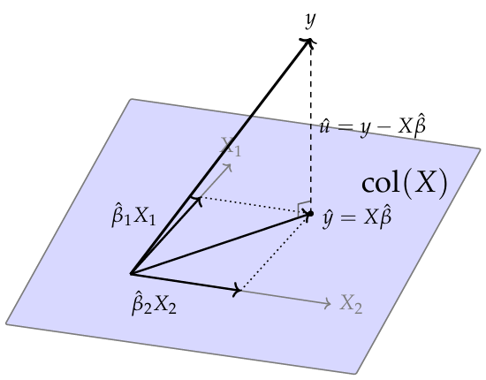
OLS minimizes \(\|\hat{u}\|^2 = \hat{u}'\hat{u}\) — the squared distance from \(y\) to \(\operatorname{col}(X)\).
Frisch–Waugh–Lovell (FWL) Theorem
The projection machinery developed above leads directly to one of the most useful algebraic results in linear regression: the Frisch–Waugh–Lovell (FWL) theorem.
FWL formalizes the concept of partialling out.
- Suppose we partition the regressor matrix as \(X = [X_1 \;\; X_2]\).
- Let \(X_1\) contain the nuisance/control regressors, and \(X_2\) contain the regressors of primary interest.
- Our objective is to estimate \(\beta_2\).
To do this, we first define the residual-maker matrix for \(X_1\): \[M_1 = I_N - X_1(X_1'X_1)^{-1}X_1'\]
Frisch–Waugh–Lovell (FWL) Theorem
Theorem — Frisch–Waugh–Lovell (FWL)
Partition \(X = [X_1 \; X_2]\). The OLS estimate of \(\beta_2\) from the full regression of \(y\) on \([X_1 \; X_2]\) equals: \[\hat\beta_2 = (\tilde{X}_2'\tilde{X}_2)^{-1}\tilde{X}_2'\tilde{y}\]
Moreover, the residuals from the full and auxiliary regressions are identical.
where, \(\tilde{X}_2\) and \(\tilde{y}\) are residualized variables, \(\tilde{X}_2 = M_1 X_2\) and \(\tilde{y} = M_1 y\).
This theorem says that the coefficient on \(X_2\) can be obtained either from the full regression or from a regression in which the linear influence of \(X_1\) has first been removed from both \(y\) and \(X_2\).
The FWL Theorem: A 3-Step Algorithm
The Frisch-Waugh-Lovell theorem is not just a mathematical curiosity; it is a highly practical algorithm for “partialling out” (or “netting out”) the effect of covariates.
To estimate the partial effect of \(X_2\) on \(y\), controlling for \(X_1\):
- Regress \(y\) on \(X_1\): Obtain the residuals \(\tilde{y} = M_1 y\). (This isolates the variation in \(y\) unexplained by \(X_1\)).
- Regress \(X_2\) on \(X_1\): Obtain the residuals \(\tilde{X}_2 = M_1 X_2\). (This isolates the variation in \(X_2\) unexplained by \(X_1\)).
- Regress \(\tilde{y}\) on \(\tilde{X}_2\): Run the regression \(\tilde{y} = \tilde{X}_2 \beta_2 + \text{residual}\).
The Core Result: The resulting OLS estimate for \(\beta_2\) from Step 3 is exactly identical to the \(\hat{\beta}_2\) obtained from the full multiple regression of \(y\) on both \(X_1\) and \(X_2\).
Decomposition of Variation and \(R^2\)
The projection results developed above also give rise to one of the most familiar summaries of regression fit.
Since \(y=\hat y+\hat u \qquad \text{and} \qquad \hat y'\hat u=0\), it follows that \[ \underbrace{y'M_{\iota}y}_{\text{TSS}} = \underbrace{\hat y'M_{\iota}\hat y}_{\text{ESS}} + \underbrace{\hat u'\hat u}_{\text{SSR}}. \]
This is the basic decomposition of variation in linear regression.
The key point is that OLS decomposes the observed variation in \(y\) into a part captured by the linear model and a part left in the residuals.
TSS \(=\sum_i (y_i-\bar y)^2\) is the total variation in the dependent variable, with \((N-1)\) degrees of freedom; ESS \(=\sum_i (\hat y_i-\bar y)^2\) is the variation accounted for by the regressors, with \((k-1)\) degrees of freedom when an intercept is included; and SSR \(=\sum_i \hat u_i^2\) is the unexplained variation, or residual variation, with \((N-k)\) degrees of freedom
\(R^2\) and Adjusted \(R^2\)
This decomposition motivates the coefficient of determination, \[ R^2 = 1-\frac{\text{SSR}}{\text{TSS}} = \frac{\text{ESS}}{\text{TSS}} \in [0,1]. \]
Thus, \(R^2\) measures the fraction of the sample variation in \(y\) that is accounted for by the linear regression model.
To account for the loss of degrees of freedom when more regressors are added: \[ \text{Adjusted }R^2 = \bar R^2 = 1-(1-R^2)\frac{N-1}{N-k}. \]
Adding an uninformative regressor may reduce \(\bar R^2\). For this reason, adjusted \(R^2\) is often more informative than \(R^2\) when comparing models with different numbers of regressors.
4. Finite-Sample Properties of OLS
Unbiasedness
Having established the algebraic mechanics of OLS, we now evaluate its statistical properties.
Is \(\hat\beta\) a reliable estimator of the true population parameter \(\beta\)? We begin by analyzing its finite-sample bias.
Recall the OLS estimator: \(\hat\beta=(X'X)^{-1}X'y\). Substituting the true data-generating process, \(y=X\beta+u\), into this expression yields: \[ \hat\beta = (X'X)^{-1}X'(X\beta + u) = \beta + (X'X)^{-1}X'u \]
Taking expectations conditional on the regressor matrix \(X\), and treating \(X\) as fixed given itself, we obtain: \[ \mathbb{E}[\hat\beta\mid X] = \beta + (X'X)^{-1}X'\mathbb{E}[u\mid X] \]
Unbiasedness
For OLS to be completely unbiased, the second term in the previous equation, \(\mathbb{E}[u\mid X]\), must vanish.
Assumption 3 — Zero Conditional Mean
\[ \mathbb{E}[u\mid X]=0 \]
That is, conditional on the full regressor matrix, the unobserved error term has a mean of exactly zero.
Note: This is arguably the most critical assumption in microeconometrics/applied econometrics (your next course). This assumption states that the regressors carry no systematic information about the unobserved shocks. So, if this assumption fails (whether due to omitted variables, measurement error, or simultaneous equations), we enter the domain of endogeneity. In this case, the second term in our derivation no longer evaluates to zero, making OLS fundamentally biased. Resolving this requires alternative identification strategies, such as Instrumental Variables.
Unbiasedness and the Variance of OLS
Under Assumptions 1, 2, and 3, OLS is conditionally unbiased: \[ \mathbb{E}[\hat\beta\mid X]=\beta. \]
This is a reassuring repeated-sampling property: across many hypothetical samples, the OLS estimator is perfectly centered at the true population parameter.
Unbiasedness alone tells us nothing about precision. An estimator can be unbiased but highly dispersed, making any single estimate unreliable. Therefore, the next crucial object of interest is the variance-covariance matrix of OLS.
Omitted Variable Bias (OVB)
What happens if the true data generating process is \(y = X_1\beta_1 + X_2\beta_2 + u\), but we mistakenly omit \(X_2\) and estimate the “short regression” \(y = X_1\tilde{\beta}_1 + v\)?
The OLS estimator for the short regression is: \[\tilde{\beta}_1 = (X_1'X_1)^{-1}X_1'y\]
Substitute the true model for \(y\): \[\tilde{\beta}_1 = (X_1'X_1)^{-1}X_1'(X_1\beta_1 + X_2\beta_2 + u)\] \[\tilde{\beta}_1 = \beta_1 + (X_1'X_1)^{-1}X_1'X_2\beta_2 + (X_1'X_1)^{-1}X_1'u\]
Taking expectations (assuming \(\mathbb{E}[u \mid X] = 0\)):
\[\mathbb{E}[\tilde{\beta}_1 \mid X] = \beta_1 + \underbrace{(X_1'X_1)^{-1}X_1'X_2}_{\text{Regression of } X_2 \text{ on } X_1} \beta_2\]
OVB occurs unless the omitted variable has no true effect (\(\beta_2 = 0\)) or the included and omitted variables are perfectly orthogonal (\(X_1'X_2 = 0\)). We will review this again in IV.
The Variance of OLS
By definition, the conditional variance of the estimator is the expected outer product of its deviation from the mean, \(\operatorname{Var}(\hat\beta\mid X) = \mathbb{E}\bigl[(\hat\beta - \beta)(\hat\beta - \beta)' \mid X\bigr]\).
Recall from our previous derivation that the estimation error is \(\hat\beta-\beta=(X'X)^{-1}X'u\). Also, we are conditioning on \(X\), so the matrices involving \(X\) are treated as non-stochastic constants. Therefore,
\[ \operatorname{Var}(\hat\beta\mid X) = (X'X)^{-1}X'\,\mathbb{E}[uu'\mid X]\,X(X'X)^{-1} \]
This is known as the “sandwich” form: The “Bread”, \((X'X)^{-1}X'\), is driven entirely by the observed regressors, and the the “Meat”, \(\mathbb{E}[uu'\mid X]\), is the \(N \times N\) covariance matrix of the unobserved errors.
To obtain the classical, mathematically tractable textbook expression (and to prove the Gauss-Markov theorem), we must introduce an additional, highly restrictive assumption about the “meat”.
Assumption 4: Spherical Disturbances
Assumption 4 — Spherical Disturbances
\[ \mathbb{E}[uu'\mid X]=\sigma^2 I_N. \]
Equivalently, conditional on \(X\), the disturbances are homoskedastic and mutually uncorrelated.
Under this assumption, the general sandwich formula collapses to \[ \operatorname{Var}(\hat\beta\mid X)=\sigma^2(X'X)^{-1}. \]
- This is the familiar variance formula from the classical linear regression model.
- The usefulness of Assumption 4 is that it gives a simple closed-form expression for the variance of OLS. The drawback is that it is often too restrictive in empirical work.
Variance of OLS and Practical Extensions
Under Assumptions 1–4, we obtain the exact finite-sample variance: \[\operatorname{Var}(\hat\beta\mid X)=\sigma^2(X'X)^{-1}\]
In empirical practice, however, the spherical-disturbance assumption (A4) frequently fails. When it does, we rely on robust “sandwich” estimators:
White’s heteroskedasticity-robust estimator: \(\widehat{\operatorname{Var}}_{rob}(\hat\beta\mid X) = (X'X)^{-1} \left( \sum_{i=1}^N \hat u_i^2 x_i x_i' \right) (X'X)^{-1}\)
Cluster-robust estimator (for within-group dependence): \(\qquad\qquad\qquad\qquad\qquad\qquad\qquad\qquad\qquad \widehat{\operatorname{Var}}_{CR}(\hat\beta\mid X) = (X'X)^{-1} \left( \sum_{g=1}^G X_g'\hat u_g\hat u_g'X_g \right) (X'X)^{-1}\)
Notes: Unlike the classical formula, these robust estimators are not exact in finite samples. They are justified entirely by large-sample asymptotic theory (which we will cover later).
Estimating \(\sigma^2\)
To make the classical variance formula feasible, we need an estimator for the unknown disturbance variance \(\sigma^2\).
The standard choice is based on the residual sum of squares: \[ \tilde\sigma^2=\frac{\hat u'\hat u}{N-k} \]
- We divide by \(N-k\) rather than \(N\). Because OLS chooses \(\hat\beta\) to minimize the sum of squared residuals, \(\hat u'\hat u\) is mechanically smaller than the true unobserved \(u'u\). This adjustment perfectly corrects for that downward bias.
- Under Assumptions 1–4, \(\mathbb{E}[\tilde\sigma^2\mid X] = \sigma^2\), so \(\tilde\sigma^2\) is an unbiased estimator of the disturbance variance (homework).
- Therefore, the feasible variance estimator of OLS is \(\widehat{\operatorname{Var}}(\hat\beta\mid X) = \tilde\sigma^2 (X'X)^{-1}\).
- In practice, the reported standard errors are simply the square roots of the diagonal elements of this estimated matrix: \[\widehat{\operatorname{se}}(\hat\beta_j) \equiv \sqrt{ \left[\widehat{\operatorname{Var}}(\hat\beta\mid X) \right]_{jj} }\]
Gauss–Markov Theorem
Theorem — Gauss–Markov (BLUE)
Under Assumptions 1–4, the OLS estimator is BLUE: the Best Linear Unbiased Estimator.
That is, for any other linear unbiased estimator \(\tilde\beta=Cy\) (where \(C\) is a matrix function of \(X\)), the difference in their variance-covariance matrices is positive semi-definite: \[ \operatorname{Var}(\tilde\beta\mid X)-\operatorname{Var}(\hat\beta\mid X)\succeq 0 \]
This guarantees that OLS is not just unbiased—it is the most efficient estimator within its class, providing the tightest possible sampling distribution.
Important: The theorem does not state that OLS is optimal among all possible estimators. It claims optimality only within the restricted class of estimators that are both linear in \(y\) and unbiased. If a researcher is willing to accept a small amount of bias (e.g., Ridge regression) or use nonlinear procedures, they may achieve a strictly lower Mean Squared Error (MSE).
Proof Sketch: Gauss–Markov Theorem
(Please refer to the Lecture Notes for the complete proof).
- Consider any arbitrary linear estimator, \(\tilde\beta=Cy\).
- We can always express its weight matrix \(C\) as the OLS weights plus some deviation matrix \(D\): \[ C=(X'X)^{-1}X'+D \]
- For \(\tilde\beta\) to be unbiased, we must have \(\mathbb{E}[Cy \mid X] = CX\beta = \beta\). This requires \(CX=I_k\). Substituting our expression for \(C\) yields: \[ \bigl((X'X)^{-1}X' + D\bigr)X = I_k + DX = I_k \quad \Longrightarrow \quad DX=0 \]
- Now, compute the conditional variance. Because \(DX=0\), the cross-terms vanish perfectly (\(DX(X'X)^{-1} = 0\)): \[ \operatorname{Var}(\tilde\beta\mid X) = \sigma^2CC' = \sigma^2(X'X)^{-1} + \sigma^2DD' \]
- Any matrix of the form \(DD'\) is positive semi-definite (\(DD'\succeq 0\)). Therefore, it mathematically follows that: \[ \operatorname{Var}(\tilde\beta\mid X) \succeq \sigma^2(X'X)^{-1} = \operatorname{Var}(\hat\beta\mid X) \]
- Conclusion: OLS strictly has the smallest variance among all linear unbiased estimators.
5. Constrained Least Squares (CLS)
Imposing Linear Restrictions
Up to this point, we have derived the OLS estimator unconditionally, allowing the data to freely dictate the parameter estimates.
In many empirical applications, however, economic theory suggests that the parameters must satisfy exact linear relationships. Common examples include:
- Constant returns to scale in a Cobb-Douglas production function (e.g., \(\beta_1 + \beta_2 = 1\)).
- Adding-up restrictions in demand systems (budget shares summing to one).
- Exclusion restrictions (forcing certain coefficients to be exactly zero).
Suppose that our parameter vector \(\beta\) is subject to \(q\) linear restrictions: \[ Q'\beta=c, \qquad Q\in\mathbb{R}^{k\times q} \text{ with full column rank}, \qquad c\in\mathbb{R}^q \]
CLS: Setup and Lagrangian
We now want to minimize the Sum of Squared Residuals (SSR) strictly over the subset of parameter values that satisfy these theoretical restrictions.
\[ \hat\beta_{CLS} = \arg\min_\beta S(\beta) \qquad \text{subject to} \qquad Q'\beta=c \]
To solve this constrained optimization problem, we set up a Lagrangian: \[ \mathcal{L}(\beta,\lambda) = (y-X\beta)'(y-X\beta) + 2\lambda'(Q'\beta-c) \] where \(\lambda\in\mathbb{R}^q\) is the vector of shadow prices (Lagrange multipliers) associated with the constraints.
Solving the first-order conditions with respect to both \(\beta\) and \(\lambda\) yields the closed-form CLS estimator: \[ \boxed{ \hat\beta_{CLS} = \hat\beta_{OLS} - (X'X)^{-1}Q\bigl[Q'(X'X)^{-1}Q\bigr]^{-1}(Q'\hat\beta_{OLS} - c) } \]
Note: The formula is often written with a plus sign by reversing the final term to \((c - Q'\hat\beta_{OLS})\).
Properties of CLS
The algebraic intuition is: it starts with the unrestricted \(\hat\beta_{OLS}\) and adjusts it by the exact minimum distance required to force the restrictions \(Q'\beta=c\) to hold.
If the unrestricted estimator happens to already satisfy the rule (\(Q'\hat\beta_{OLS}=c\)), the adjustment term evaluates to zero and \(\hat\beta_{CLS}=\hat\beta_{OLS}\).
The statistical properties depend entirely on whether the imposed theory is true:
- If the restrictions are CORRECT: (i) CLS remains perfectly unbiased; (ii) CLS is more efficient than unrestricted OLS (its variance is smaller in the positive semi-definite matrix sense).
- If the restrictions are FALSE: (i) CLS becomes fundamentally biased; (ii) We face a harsh bias-variance tradeoff: we gain mechanical efficiency (smaller variance) but force the estimator to converge to the wrong parameter values, causing misspecification.
Because imposing false restrictions damages the consistency of our estimator, we must formally test whether the data supports the theory. This leads us directly to the \(F\)-test.
6. Inference in OLS
Assumption 5: Normality
Up to this point, the Gauss–Markov theorem guaranteed that OLS is BLUE relying only on assumptions about the conditional mean and variance.
However, obtaining a point estimate is not enough. We are also interested in inference. To conduct hypothesis tests and compute exact tail probabilities in finite samples, we must fully specify the data-generating process.
To conduct exact finite-sample inference, we add a distributional assumption to the classical linear model:
Assumption 5 — Normality
\[ u \mid X \sim \mathcal{N}(0,\sigma^2 I_N) \]
Distributional Results
The normal linear regression model is theoretically elegant because the linear algebra of OLS maps directly into standard probability distributions.
Under Assumptions 1–5:
(i) \[ \hat\beta \mid X \sim \mathcal{N}\!\bigl(\beta,\;\sigma^2(X'X)^{-1}\bigr) \]
(ii) \[ \frac{\hat u'\hat u}{\sigma^2} \sim \chi^2(N-k) \]
(iii) \(\hat\beta\) and \(\hat u'\hat u\) are independent conditional on \(X\).
Distributional Results
Why are these results true?
(i) Under normality, the estimator \(\hat\beta=\beta+(X'X)^{-1}X'u\) is strictly a linear transformation of a normal vector, which is always normally distributed.
(ii) The residual sum of squares can be written as a quadratic form in the idempotent matrix \(M\): \(\hat u'\hat u=u'Mu\). Because \(M\) has rank \(N-k\), this maps to the sum of \(N-k\) squared independent standard normal variables.
(iii) The estimator depends on \(u\) through \((X'X)^{-1}X'u\), while the residuals depend on \(u\) through \(Mu\). Since \(X'M=0\), these components are orthogonal; under joint normality, zero covariance (orthogonality) guarantees strict independence.
Homework: Prove (ii) and (iii) rigorously using the spectral decomposition of the idempotent matrix \(M\).
The \(t\)-Test
Suppose we want to test a null hypothesis on a single coefficient: \[ H_0:\beta_j=\beta_{j,0} \]
From the corollary above, we know the exact distribution of that specific coefficient: \[ \hat\beta_j \mid X \sim \mathcal{N}\!\bigl(\beta_j,\;\sigma^2[(X'X)^{-1}]_{jj}\bigr) \]
- If the population variance \(\sigma^2\) were known, we could construct a standard normal \(Z\)-statistic. Because it is unknown, we replace it with our unbiased estimator \(\tilde\sigma^2\).
- That replacement matters because \(\tilde\sigma^2\) is itself a random variable. The feasible statistic becomes the ratio of a standard normal variable to the square root of an independent \(\chi^2\) variable (divided by its degrees of freedom). This exact construction defines a Student-\(t\) distribution.
The \(t\)-Test
Therefore, the feasible test statistic is: \[ t_j=\frac{\hat\beta_j-\beta_{j,0}}{\sqrt{\tilde\sigma^2[(X'X)^{-1}]_{jj}}} \sim t_{N-k} \qquad \text{under } H_0 \]
The decision rule is to reject \(H_0\) at significance level \(\alpha\) if \(|t_j| > t_{N-k,\alpha/2}\).
A particularly common application is testing \(H_0:\beta_j=0\), which determines whether regressor \(j\) has a statistically discernible effect distinct from zero.
The \(F\)-Test and Wald Test
Now consider testing multiple restrictions simultaneously with a joint null hypothesis: \[ H_0:Q'\beta = c \] where \(Q\) is a \(k\times q\) matrix of rank \(q\) (matching our setup from Constrained Least Squares).
The \(F\)-test asks whether imposing these \(q\) linear restrictions makes the model fit the data substantially worse. The classical \(F\)-statistic compares the restricted and unrestricted Sum of Squared Residuals (SSR): \[ F = \frac{(\text{SSR}_R-\text{SSR}_U)/q}{\text{SSR}_U/(N-k)} \sim F_{q,N-k} \qquad \text{under } H_0 \]
The \(F\)-Test and Wald Test
An equivalent formulation uses only the unrestricted estimates. This is the Wald form: \[ F_W = \frac{(Q'\hat\beta - c)'\bigl[Q'(X'X)^{-1}Q\bigr]^{-1}(Q'\hat\beta - c)}{\tilde\sigma^2\,q} = F \]
This statistic is numerically identical to the SSR-based \(F\)-statistic.
The interpretation is intuitive: it measures how far the unrestricted estimates \(Q'\hat\beta\) are from the hypothesized values \(c\), weighted by the precision (variance-covariance) of those estimates.
Asymptotic Connection
Under Assumption 5 (Normality), we know that exactly: \[ F_W \sim F_{q,N-k} \]
It is theoretically useful to define the corresponding Wald statistic (without dividing by \(q\)): \[ W = q\cdot F_W \]
In large samples, even if the normality assumption fails, the Central Limit Theorem ensures that: \[ W \xrightarrow{d} \chi^2(q) \]
This is why the Wald principle extends so naturally to asymptotic inference later in the course.
The \(p\)-Value
The previous slides presented hypothesis testing in its critical-value form.
The \(p\)-value expresses the exact same logic from a different angle.
Observed significance level: The \(p\)-value is the probability of obtaining a test statistic at least as extreme as the one actually observed in the sample: \[ p\text{-value}=\Pr_{H_0}(\text{statistic at least as extreme as observed}) \]
For the two-sided \(t\)-test, this becomes: \[ p\text{-value} = 2\Pr(t_{N-k}\ge |t_{\text{obs}}|) = 2\bigl[1-F_{t_{N-k}}(|t_{\text{obs}}|)\bigr] \]
The \(p\)-Value
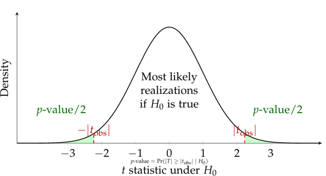
Equivalently, the decision rule simplifies to: \[ \text{Reject } H_0 \text{ at level } \alpha \qquad \Longleftrightarrow \qquad p\text{-value} < \alpha \]
7. OLS and Gaussian Quasi-MLE
Connection to Maximum Likelihood
Under Assumption 5 (Normality), the conditional density of \(y_i\) given \(x_i\) is strictly normal.
We will formally study Maximum Likelihood Estimation (MLE) later in the course. But, by now, we can take advantage of our current assumption.
Let’s introduce a fundamental mathematical object: the conditional log-likelihood function for the entire sample of \(N\) independent observations.
Because the observations are independent, the joint log-likelihood is simply the sum of the individual log-densities. In matrix notation, this is: \[ \ell_N(\beta,\sigma^2 \mid y, X) = -\frac{N}{2}\ln(2\pi) - \frac{N}{2}\ln(\sigma^2) - \frac{1}{2\sigma^2}(y - X\beta)'(y - X\beta) \]
The Conditional Log-Likelihood
Notice that the final term contains the exact OLS objective function, \(S(\beta) = (y - X\beta)'(y - X\beta)\).
We can elegantly rewrite the log-likelihood as: \[ \ell_N(\beta,\sigma^2 \mid y, X) = \text{const} - \frac{1}{2\sigma^2}S(\beta) \]
Because the variance \(\sigma^2\) is strictly positive, maximizing this log-likelihood with respect to \(\beta\) is mathematically identical to minimizing the sum of squared residuals \(S(\beta)\). Therefore, under normality, OLS and MLE are exactly the same estimator for \(\beta\).
Gaussian Quasi-MLE (QMLE)
If we incorrectly assume normality (Assumption 5 fails) and maximize the Gaussian likelihood function anyway, this is known as Gaussian Quasi-Maximum Likelihood Estimation (QMLE).
Because the first-order conditions for \(\beta\) in the Gaussian likelihood depend only on the linear residuals, maximizing this “wrong” likelihood still perfectly yields the OLS estimator for \(\beta\).
This is a profound theoretical result:
- The consistency of the OLS estimator for the conditional mean does not depend on the normality assumption.
- This establishes the foundation for Quasi-Likelihood methods later in the course.
For example, in count data, maximizing a Poisson likelihood (even if the true data is not Poisson-distributed) will still yield consistent parameter estimates as long as the conditional mean is correctly specified.
8. Information Criteria
Model Selection: Information Criteria (AIC and BIC)
Although we have already presented \(R^2\) and \(\bar{R}^2\), I will now introduce an alternative approach. To do so, we must first understand the fundamental trade-off in econometrics: Goodness of Fit vs. Parsimony.
- Adding more variables always increases (or maintains) \(R^2\), but it risks overfitting the model to noise rather than signal.
- Information Criteria provide a “penalty” for complexity, allowing us to compare models that are not necessarily nested.
- It helps when choosing between different sets of independent variables.
AIC and BIC: Mathematical Definition
Under the assumption of Gaussian disturbances, we calculate these criteria based on the Sum of Squared Residuals (\(\hat{u}'\hat{u}\)), the sample size (\(n\)), and the number of parameters (\(k\)):
\[ \mathrm{AIC}=n\ln\left(\frac{\hat u'\hat u}{n}\right)+2k \]
\[ \mathrm{BIC}=n\ln\left(\frac{\hat u'\hat u}{n}\right)+k\ln n \]
Note: In both cases, the model with the lowest value is preferred.
Strategic Comparison
While both metrics penalize the inclusion of extra variables, they do so with different intensities:
- AIC (Akaike): The penalty (\(2k\)) is constant. It tends to be more “generous” and often favors richer models (more parameters).
- BIC (Bayesian): The penalty (\(k \ln n\)) depends on the sample size. Since \(\ln n > 2\) for any \(n > 7\), BIC penalizes complexity more heavily than AIC.
Note
These criteria are powerful automated tools for model selection, but they do not replace economic theory.
9. Prediction and Forecast Evaluation
Plug-in Predictor and Uncertainty
Given a newly observed covariate vector \(x_{N+j}\), the natural out-of-sample predictor simply replaces the unknown parameters with our OLS estimates: \[ \hat{y}_{N+j} = x_{N+j}'\hat\beta \]
When forecasting, we must clearly distinguish between two different prediction targets, each with different sources of uncertainty:
- Targeting the Conditional Mean: \(\mathbb{E}[y_{N+j} \mid x_{N+j}] = x_{N+j}'\beta\)
- Source of error: Purely estimation uncertainty (because \(\hat\beta \neq \beta\)).
- Targeting the Realized Outcome: \(y_{N+j} = x_{N+j}'\beta + u_{N+j}\)
- Source of error: Estimation uncertainty PLUS the irreducible future shock (\(u_{N+j}\)).
Mean Squared Forecast Error (MSFE)
To quantify the precision of our prediction for the realized outcome (under the assumption of homoskedasticity), we compute the MSFE:
\[ \mathbb{E}\bigl[(\hat{y}_{N+j} - y_{N+j})^2 \mid x_{N+j}\bigr] = \sigma^2 \bigl[ 1 + x_{N+j}'(X'X)^{-1}x_{N+j} \bigr] \]
This elegantly decomposes the forecast variance into two distinct parts: * \(\sigma^2 \times 1\): The irreducible fundamental uncertainty from the future shock \(u_{N+j}\). No matter how much data we have, this remains. * \(\sigma^2 \times x_{N+j}'(X'X)^{-1}x_{N+j}\): The estimation uncertainty.
Geometric Intuition: Notice that the estimation uncertainty depends on a quadratic form of \(x_{N+j}\). This means that predicting outcomes for covariate profiles that are very far from the historical sample average will mechanically result in much larger forecast standard errors.
Forecast Evaluation Metrics
Once out-of-sample predictions are generated, how do we evaluate model performance over \(J\) hold-out periods?
Common accuracy measures:
| Measure | Formula | Notes |
|---|---|---|
| RMSE | \(\sqrt{\frac{1}{J}\sum_{j=1}^J (\hat{y}_{N+j} - y_{N+j})^2}\) | Scale-dependent; quadratically penalizes large errors. |
| MAE | \(\frac{1}{J}\sum_{j=1}^J |\hat{y}_{N+j} - y_{N+j}|\) | Scale-dependent; penalizes linearly, more robust to outliers. |
| Theil’s \(U\) | Normalized RMSE ratio | Dimensionless; often compares the model against a naive “random walk” baseline. |
Cierre

\[\,\]
luis.chanci@usach.cl
luischanci@santotomas.cl