2×4 Matrix{Float64}:
2.19355 0.425284 5.15785 0.0355944
0.233871 0.0296309 7.8928 0.0156759Computational Methods in Econometrics
Magíster en Economía
Teoría Econométrica (Econometric Theory)
Prof. Luis Chancí
Outline
- Introduction: Why a Computational Chapter?
- From Theory to Computation
- OLS as Matrix Algebra:
- Reviewing The Notation
- A Small Numerical Example
- Programming OLS from scratch in R and Julia
- From Pencil-and-Paper to R, Julia, and Stata
- OLS as Matrix Algebra:
- OLS as an optimization problem
- Monte Carlo simulation
- Bootstrap resampling
Main idea: move from the theory of estimators to their computational implementation, evaluation, and practical inference.
1. Introduction
Introduction: Why a Computational Chapter?
The previous notes established the theory of OLS: unbiasedness, efficiency under classical assumptions, and inference.
This chapter asks a different question:
How do we actually compute, study, and use an estimator in practice?
Three motivations:
- formulas must be translated into reproducible code
- many estimators have no closed-form solution
- simulation and resampling let us study finite-sample behavior when theory is hard or only asymptotic
The Logic of the Chapter
All the topics in this chapter are connected.
- Programming OLS shows how the algebra becomes code (I will use Julia, R and Stata).
- Optimization shows that OLS is an extremum estimator.
- Monte Carlo studies how estimators behave across repeated samples (Simulations)
- Bootstrap approximates sampling uncertainty using the data themselves: a procedure for estimating the distribution of an estimator by resampling.
This is not a separate branch of econometrics. It is the practical side of the same theory.
2. From Theory to Computation
OLS as Matrix Algebra: Reviewing The Notation
Let \(k=2\) and \(i=1,\ldots,n\), the linear model is: \[Y_i=\beta_1+\beta_2 X_i+u_i\] Using matrix notation: \[\left[ \begin{array}{c} Y_1\\ \vdots \\ Y_n\\ \end{array} \right] = \left[ \begin{array}{c} \beta_1+\beta_2 X_1+u_1\\ \vdots \\ \beta_1+\beta_2 X_n+u_n\\ \end{array} \right] = \left[ \begin{array}{c} \beta_1+\beta_2 X_1\\ \vdots\\ \beta_1+\beta_2 X_n\\ \end{array} \right]+\left[ \begin{array}{c} u_1\\ \vdots\\ u_n\\ \end{array} \right]\]
In other words, \[\left[ \begin{array}{c} Y_1\\ \vdots\\ Y_n\\ \end{array}\right]_{nx1}= \left[\begin{array}{cc} 1 & X_1\\ \vdots \\ 1 & X_n\\ \end{array} \right]_{nx2} \cdot \left[\begin{array}{c} \beta_1\\ \beta_2\\ \end{array}\right]_{2x1} + \left[ \begin{array}{c} u_1\\ \vdots\\ u_n\\ \end{array} \right]_{nx1} \hspace{0.5cm}\Rightarrow\hspace{0.5cm} \underbrace{Y}_{(n\,x\,1)}=\underbrace{X}_{(n\,x\,2)}\underbrace{\beta}_{(2\,x\,1)}+\underbrace{u}_{(n\,x\,1)}\]
OLS as Matrix Algebra: Reviewing The Notation (2)
Generally speaking, for \(k\) regressors and \(i=1,\ldots,n\),
\[Y_i=\beta_1+\beta_2 X_{2i}+...+\beta_k X_{ki}+u_i\] thus,
\[\left[\begin{array}{c} Y_1\\ \vdots\\ Y_n\\ \end{array}\right]=\left[ \begin{array}{c} \beta_1+\beta_2 X_{21}+...+\beta_k X_{k1}+u_1\\ \vdots\\ \beta_1+\beta_2 X_{2n}+...+\beta_k X_{kn}+u_n\\ \end{array}\right]\]
which means \[\left[\begin{array}{c} Y_1\\ \vdots\\ Y_n\\ \end{array}\right]_{nx1}= \left[\begin{array}{cccccc} 1 & X_{21}& .&.&.&X_{k1}\\ \vdots\\ 1 & X_{2n}& .&.&.&X_{kn}\\ \end{array}\right]_{nxk} \left[\begin{array}{c} \beta_1\\ \vdots\\ \beta_k\\ \end{array}\right]_{kx1} +\left[\begin{array}{c} u_1\\ \vdots\\ u_n\\ \end{array}\right]_{nx1} \hspace{0.5cm}\Rightarrow\hspace{0.5cm} \underbrace{Y}_{(n\,x\,1)}=\underbrace{X}_{(n\,x\,k)}\underbrace{\beta}_{(k\,x\,1)}+\underbrace{u}_{(n\,x\,1)}\]
OLS as Matrix Algebra: A summary of equations.
We found that the OLS estimator is \[ \hat\beta=(X'X)^{-1}X'Y. \]
The fitted values and residuals are \[ \hat Y=X\hat\beta, \qquad \hat u=Y-\hat Y. \]
Under homoskedasticity, \[ \widehat{\operatorname{Var}}(\hat\beta\mid X)=\hat\sigma^2(X'X)^{-1}, \qquad \hat\sigma^2=\frac{\hat u'\hat u}{n-k}. \] And inference is based on normality. For instance,
\[\frac{\hat{\beta}_j}{\sqrt{\widehat{\text{Var}}_{jj}(\hat{\boldsymbol{\beta}}|\boldsymbol{X})}}\,\sim\,t\text{-student}_{[\alpha/2;(n-k)]} \hspace{0.5cm}\text{, or,}\hspace{0.5cm} \frac{(R\hat{\beta}-r)'\left[ \sigma^2R(X'X)^{-1}R' \right]^{-1} (R\hat{\beta}-r)/q}{\hat{u}'\hat{u}/(n-k)}\sim F_{[q,(n-k)]} \]
A Small Numerical Example
Consider the data \[\begin{array}{l|cccc} Y& 2 & 5 & 6 & 7\\ \hline X& 0 & 10 & 18 & 20\\ \end{array}\]
That is, the linear model is \(Y_i=\hat{\beta}_1+\hat{\beta}_2X_i+\hat{u}_i\) and \(k=2\), \[\begin{array}{ccccccccc} 2&=&\hat{\beta}_1&+&\hat{\beta}_2&*&0&+&\hat{u}_1\\ 5&=&\hat{\beta}_1&+&\hat{\beta}_2&*&10&+&\hat{u}_2\\ & & & &\vdots & & & & \\ \end{array}\]
Using matrix algebra
\[\left[\begin{array}{c} 2 \\ 5 \\ 6 \\ 7\\ \end{array} \right]= \left[\begin{array}{cc} 1&0 \\ 1&10 \\ 1&18 \\ 1&20\\ \end{array} \right] \left[\begin{array}{c} \hat{\beta}_1 \\ \hat{\beta}_2\\ \end{array} \right]+ \left[\begin{array}{c} \hat{u}_1 \\ \hat{u}_2 \\ \hat{u}_3 \\ \hat{u}_4\\ \end{array} \right] \hspace{0.6cm}\rightarrow \underbrace{Y}_{(4x1)}=\underbrace{X}_{(4x2)}\underbrace{\hat{\beta}}_{(2x1)}+\underbrace{\hat{u}}_{(4x1)}\]
A Small Numerical Example
Then
\[\begin{eqnarray*} \hat{\beta}&=& \left(\begin{array}{c} \hat{\beta}_1\\ \hat{\beta}_2\\ \end{array}\right)= \left( \left[\begin{array}{cccc} 1&1&1&1\\ 0&10&18&20\\ \end{array} \right] \left[\begin{array}{cc} 1&0 \\ 1&10 \\ 1&18 \\ 1&20\\ \end{array} \right] \right)^{-1} \left( \left[\begin{array}{cccc} 1&1&1&1\\ 0&10&18&20\\ \end{array} \right] \left[\begin{array}{c} 2 \\ 5 \\ 6 \\ 7\\ \end{array} \right] \right)= \left(\frac{1}{992} \left[\begin{array}{cc} 824 & -48 \\ -48 & 4\\ \end{array}\right]\right) \left(\left[\begin{array}{c} 20\\ 298\\ \end{array}\right]\right)= \left(\begin{array}{c} 2,1935\\ 0,2338\\ \end{array}\right) \end{eqnarray*}\]
So the fitted line is \(\hat Y_i=2.1935+0.2338X_i\). And the (fitted) residuals,
\[\hat{u}= \left[\begin{array}{c} \hat{u}_1 \\ \hat{u}_2 \\ \hat{u}_3 \\ \hat{u}_4 \\ \end{array}\right]=Y-X\hat{\beta}= \left[\begin{array}{c} 2 \\ 5 \\ 6 \\ 7\\ \end{array}\right]- \left[\begin{array}{cc} 1&0 \\ 1&10 \\ 1&18 \\ 1&20\\ \end{array} \right] \left[\begin{array}{c} 2,1935\\ 0,2339\\ \end{array}\right]= \left[\begin{array}{c} -0.1935 \\ \,\,0.4677 \\ -0.4032 \\ \,\,0.1290 \end{array}\right]\]
And the estimate of \(\sigma^2\): \[\hat{\sigma}^{2}=\frac{\sum_{i=1}^{4}\hat{u}_i^{2}}{n-k}=\frac{(-0.1935)^2+(0.4677)^2+(-0.4032)^2+(0.1290)^2}{4-2}=\frac{0.4355}{2}\simeq0.218\]
Same Example: Residuals and Inference
\[Var(\hat{\beta}|X)=\hat{\sigma}^{2}(X'X)^{-1}=\frac{0.4355}{2} \left[\begin{array}{cc} 4&48 \\ 48& 824\\ \end{array} \right]^{-1}\simeq \left[\begin{array}{cc} 0.1809&-0.0105 \\-0.0105& 0.0008789\\ \end{array} \right]\]
Thus, the inference, \(H_0:\beta_j=0\) vs \(H_1:\beta_j\neq0\); using \(t^{c}_{\alpha/2;n-k}=t^{c}_{0.025;2}=4,3027\),
- For \(\hat{\beta}_1\): \(t_{\hat{\beta}_1}=\frac{2,1935}{\sqrt{0.1809}}=5.158\). As \(t_{\hat{\beta}_1}>t^{c}_{0.025;2}\) we reject \(H_0\); In other words, \(\hat{\beta}_1\) is statistically significant at the \(95\%\).
- For \(\hat{\beta}_2\): \(t_{\hat{\beta}_2}=\frac{0,2338}{\sqrt{0.0008789}}=7.893\). As \(t_{\hat{\beta}_2}>t^{c}_{0.025;2}\) we reject \(H_0\); in other words, \(\hat{\beta}_2\) is statistically significant at the \(95\%\).
The \(R^{2}\) is constructed using \(STC=\sum y_i^{2}=\sum (Y_i-\bar{Y})^2=\sum (Y_i-5)^2=14\), \[R^{2}=1-\frac{SRC}{STC}=1-\frac{\sum\hat{u}_i^2}{\sum y_i^2}=1-\frac{0.4355}{14}=0.969 \hspace{0.5cm};\hspace{0.5cm} \bar{R}^{2}=1-\frac{\sum\hat{u}_i^2/(n-k)}{\sum y_i^2/(n-1)}=1-\frac{0.4355/2}{14/3}=0.9533\]
Programming OLS
Why Program OLS from Scratch (e.g, using R, Julia, or Python)?
Built-in commands such as lm() in R or reg in Stata are very convenient, but they hide the underlying computational logic. Also, once we add modifications to an estimator, we may not be able to rely on a pre-programmed command.
Programming OLS directly is useful because it:
- reveals how the estimator is actually computed
- makes matrix formulas operational
- prepares us to code new estimators not available in standard software
Once you can code OLS from scratch, you are much closer to coding IV, GMM, MLE, or bootstrap estimators.
From Pencil-and-Paper to R
Using
  # Ingreso de datos
  Y <- c(2,5,6,7)
  X <- cbind(rep(1,4),c(0,10,18,20))

  n <- nrow(X)
  k <- ncol(X)

  # Computo usando matrices
  Beta <- solve(t(X)%*%X)%*%(t(X)%*%Y)
  u    <- Y - X%*%Beta
  s2   <- t(u)%*%u / (n-k)
  V.b  <- as.numeric(s2)*solve(t(X)%*%X)
  t.b  <- Beta / sqrt(diag(V.b))
  p.b  <- 2*( 1 - pt(abs(t.b),(n-k)) )

  # Resultados
  # Beta hat, s.e. , t-values, p-values
cbind(Beta,sqrt(diag(V.b)),t.b,p.b) The code is almost a literal transcription of the matrix algebra.
From Pencil-and-Paper to R (cont.)
Alternative: OLS with the lm() Function in
RObject{S4Sxp}
+-------------+--------+-------+-------+-------+
|             | (1)                            |
+-------------+--------+-------+-------+-------+
|             | Est.   | S.E.  | t     | p     |
+=============+========+=======+=======+=======+
| (Intercept) | 2.194  | 0.425 | 5.158 | 0.036 |
+-------------+--------+-------+-------+-------+
| x_data      | 0.234  | 0.030 | 7.893 | 0.016 |
+-------------+--------+-------+-------+-------+
| Num.Obs.    | 4      |       |       |       |
+-------------+--------+-------+-------+-------+
| R2          | 0.969  |       |       |       |
+-------------+--------+-------+-------+-------+
| R2 Adj.     | 0.953  |       |       |       |
+-------------+--------+-------+-------+-------+
| AIC         | 8.5    |       |       |       |
+-------------+--------+-------+-------+-------+
| BIC         | 6.6    |       |       |       |
+-------------+--------+-------+-------+-------+
| Log.Lik.    | -1.241 |       |       |       |
+-------------+--------+-------+-------+-------+
| F           | 62.296 |       |       |       |
+-------------+--------+-------+-------+-------+
| RMSE        | 0.33   |       |       |       |
+-------------+--------+-------+-------+-------+
From Pencil-and-Paper to Julia

# Ingreso de datos
Y = [2,5,6,7];
X = [ones(4) [0,10,18,20]];

n, k = size(X);

# Computo usando matrices
using LinearAlgebra;
Beta = (X'X)\(X'Y); # Es preferible a inv(X'X)*X'Y por estabilidad numérica
u    = Y - X * Beta;
s2   = (u'*u) / (n - k);
Vb   = s2[1] * inv(X'*X);
tb   = Beta ./ sqrt.(diag(Vb));

using Distributions; # La librería Distributions es para el p-value
d   = TDist(n - k);
pb  = 2 .* (1 .- cdf.(d, abs.(tb)));

[Beta sqrt.(diag(Vb)) tb pb] # Beta hat, s.e. , t-values, p-values
2×4 Matrix{Float64}:
2.19355 0.425284 5.15785 0.0355944
0.233871 0.0296309 7.8928 0.0156759From Pencil-and-Paper to Stata

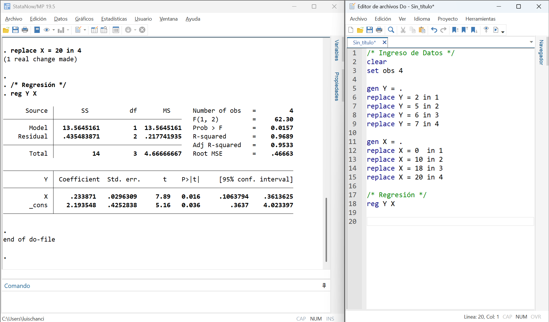
3. OLS as Optimization
OLS as an Extremum Estimator
Remember that OLS is not just a formula. It is the solution to an optimization problem:
\[\hat{\boldsymbol{\beta}}=\text{arg min}_{\beta}\,L_i(f_{\beta}(\boldsymbol{X}_i,\boldsymbol{\beta}),Y_i)\]
Alternatively, we can say that it minimizes a loss function \(S(\beta)\) based on squared residuals:
\[ \hat\beta=\operatorname*{arg\,min}_{\beta} S(\beta), \qquad S(\beta)=(Y-X\beta)'(Y-X\beta). \]
This interpretation matters because many estimators studied later (like MLE or GMM) do not have closed-form solutions and must be obtained numerically.
Numerical Unconstrained Optimization
In this section, we discuss numerical methods for optimizing an objective function when no closed-form solution is available—that is, when we cannot simply differentiate the objective function, set the first-order condition equal to zero, and solve for the parameter.
We will focus on two foundational iterative methods:
- Newton’s Method (Newton-Raphson)
- Gradient Descent (Steepest Descent)
To build intuition, let’s start with a simple optimization in one dimension. Assume \(f(z)\) is a twice continuously differentiable function (\(C^2\)): \[ \min_{z \in \mathbb{R}} f(z) \]
Newton’s Method
The intuition of Newton’s Method is to use a second-order Taylor approximation of \(f(z)\) at our current guess \(a\) \[p(z) \approx f(a) + f'(a)(z - a) + \frac{f''(a)}{2}(z - a)^2\]
- We approximately minimize \(f\) by minimizing the quadratic polynomial \(p(z)\).
- If \(f''(a) > 0\) (the function is strictly convex locally), the minimum of \(p(z)\) occurs where the derivative is zero, yielding the update rule: \(z_m = a - f'(a)/f''(a)\).
Algorithm: Newton’s Method in \(\mathbb{R}^1\)
Initialize. Choose an initial guess \(z_0\) and stopping parameters \(\delta, \epsilon > 0\).
- Step 1. Update the guess: \(z_{k+1} = z_k - \frac{f'(z_k)}{f''(z_k)}\).
- Step 2. Check convergence: If \(|z_k - z_{k+1}| < \epsilon\) and \(|f'(z_{k+1})| < \delta\), STOP and report success.
- Step 3. Else, set \(k = k+1\) and go back to Step 1.
Direction Set Methods & Gradient Descent
- Problem with Newton’s: It requires second derivatives (the Hessian matrix in higher dimensions), which can be computationally expensive to calculate and invert, or unstable if the function isn’t globally convex.
- Alternative Solution: If we simply look at the slope and always move downhill (opposite to the gradient), we will eventually reach a local minimum.
Algorithm: Gradient Descent
Initialize. Choose an initial \(z_0\), a tolerance \(\epsilon > 0\), and a learning rate \(\eta > 0\).
- Step 1. Compute the search direction (steepest downhill): \(s_k = -f'(z_k)\).
- Step 2. Determine the step size \(\lambda_k\). (In classical optimization, we might perform an exact line search: \(\lambda_k = \arg\min_\lambda f(z_k + \lambda s_k)\). In modern applications, we usually just set a fixed learning rate: \(\lambda_k = \eta\)).
- Step 3. Update the guess: \(z_{k+1} = z_k + \lambda_k s_k \quad\) (i.e., \(z_{k+1} = z_k - \eta f'(z_k)\)).
- Step 4. Check convergence: If \(|| z_k - z_{k+1} || < \epsilon\), STOP and report success; else go to Step 1.
Note: In the classical numerical optimization literature, moving in the exact opposite direction of the gradient is called Steepest Descent. In modern Machine Learning, this exact same algorithm is universally known as Gradient Descent (GD), and it forms the backbone of training deep neural networks.
Gradient Descent for OLS
Gradient descent in the case of OLS updates the parameter vector by moving against the gradient: \[ \beta^{(t+1)}=\beta^{(t)}-\eta\nabla_\beta S(\beta^{(t)}) \]
Given that the gradient is \(\nabla_\beta S(\beta) = -2X'Y + 2X'X\beta = -2X'(Y-X\beta)\), the update rule becomes:
\[ \beta^{(t+1)}=\beta^{(t)}+2\eta X'(Y-X\beta^{(t)}) \]
Thus, Gradient Descent shows that an estimator can be computed iteratively even without a closed-form formula.
A Short R Implementation
# Initialize Parameters
beta_0  <- c(0, 0)                 # Initial guess z_0
eta     <- 0.001                   # Learning rate (step size lambda)
epsilon <- 1e-6                    # Stopping parameter for parameter change
maxit   <- 1e3                     # Safeguard against infinite loops

for (k in 1:maxit) {               # Gradient Descent Loop
  grad     <- -2*crossprod(X, (Y - X%*%beta_0)) # Compute the search direction (Gradient)
  beta_new <- beta_0 - eta * grad               # Update the guess (Move downhill)

  if (max(abs(beta_new - beta_0)) < epsilon) {  # Check for convergence
    cat("STOP and report success. Converged at iteration:", k, "\n")
    beta_0 <- beta_new
    break
  }
  beta_0 <- beta_new                           # Prepare for next iteration
}

cat("Estimated Betas: ", round(beta_0, 4), "\n")
Estimated Betas: 1.997 0.2453 The algorithm starts from a guess and keeps improving it until the gradient is arbitrarily close to zero.
Newton’s Method for OLS
Newton’s method uses both first and second derivatives (the Hessian), so in the case of OLS we have: \[ \beta^{(t+1)}=\beta^{(t)}-[H(\beta^{(t)})]^{-1}\nabla_\beta S(\beta^{(t)}). \]
Since for OLS, the Hessian is constant: \[ H(\beta)=2X'X \] Substituting this into the update rule means that one Newton step yields: \[ \beta^{(t+1)}=(X'X)^{-1}X'Y=\hat\beta_{OLS} \]
Because the OLS objective is a perfect quadratic bowl, Newton’s method reaches the exact global minimum in one step from any starting value.
Using R: The optim() Function
Alternative: Optimize a function without writing the loop manually in
# Define the Objective Function (SSR)
ssr_fn <- function(beta) {
  sum((Y - X %*% beta)^2)
}

initial_guess <- c(0, 0)

# Run the optimization using "BFGS",
# a popular quasi-Newton method.
optim(
  par = initial_guess,       # Starting values
  fn = ssr_fn,               # The objective function to minimize
  method = "BFGS"            # Optimization algorithm
)
OrderedCollections.OrderedDict{Symbol, Any} with 5 entries:
:par => [2.19355, 0.233871]
:value => 0.435484
:counts => [36, 9]
:convergence => 0
:message => nothingUsing Julia
using Optim

# Define the Objective Function (SSR)
ssr_fn(beta) = sum((Y - X * beta).^2)

initial_guess = [0.0, 0.0]

# Run the optimization
result = optimize(
         ssr_fn,          # The objective function to minimize
         initial_guess,   # Starting values
         BFGS()           # Optimization algorithm
         )

println(
  "Estimated Betas: ",
  round.(Optim.minimizer(result),
         digits=4))
Estimated Betas: [2.1935, 0.2339]
Using Julia

Final Comments on Optimization
Before concluding this section, we will briefly bridge the gap between classical econometrics and modern computational methods:
- Non-Linear Least Squares (NLLS): A canonical example of an objective function requiring numerical optimization, as it lacks the analytical closed-form solution of OLS.
- The Machine Learning Connection: How modern prediction techniques (like Neural Networks) naturally extend the NLLS framework from an econometric perspective.
- Automatic Differentiation (AD): A computational tool that makes calculating derivatives for complex, high-dimensional functions practically effortless.
We will cover NLLS in more detail in the next section of the course as an extension of OLS, alongside other methods like GLS, LASSO, and Ridge regression.
From OLS to Non-Linear Least Squares (NLLS)
Suppose the conditional expectation function is non-linear in its parameters: \[ y_i=m(x_i,\beta)+u_i, \qquad \mathbb{E}[u_i\mid x_i]=0 \]
To estimate \(\beta\), we minimize the sum of squared residuals, giving the NLLS estimator: \[ \hat\beta_{NLLS}=\operatorname*{arg\,min}_\beta \sum_{i=1}^n \bigl(y_i-m(x_i,\beta)\bigr)^2 \]
Notice that OLS is simply the special case where the function is strictly linear: \(m(x_i,\beta)=x_i'\beta\).
The Key Difference: The optimization logic remains exactly the same. However, because the first-order conditions are now non-linear, analytical solutions are rarely possible. Numerical methods are no longer optional—they are mandatory.
NLLS and Modern Machine Learning
Many modern predictive models, including deep learning, are fundamentally large-scale non-linear least squares problems.
For example, a simple feedforward neural network (with one hidden layer) can be written as: \[ m(x_i,\theta)=\alpha_0+\alpha'x_i+\sum_{j=1}^q \gamma_j G(x_i'\delta_j) \] (where \(G(\cdot)\) is a non-linear activation function, and \(\theta\) collects all parameters).
- The regression function is highly non-linear in its parameters.
- Estimation still relies on minimizing a loss function (e.g., squared error).
- Numerical optimization (like Gradient Descent) entirely replaces closed-form algebra.
The Econometric Perspective: Neural networks are essentially highly flexible, non-linear function approximators. They extend the traditional NLLS framework into high dimensions rather than replacing the underlying statistical logic.
A Computational Note: Automatic Differentiation
For OLS, taking the derivative of the objective function by hand is trivial. For complex non-linear models or deep neural networks, manual derivation is error-prone and computationally inefficient.
Automatic Differentiation (AD) solves this by computing exact derivatives algorithmically. It breaks down complex functions into elementary operations and systematically applies the chain rule.
This tool is essential for:
- Estimating complex, highly non-linear econometric models.
- High-dimensional optimization where the gradient vector is massive.
- Powering modern machine-learning frameworks (e.g., PyTorch, TensorFlow, or Flux.jl in Julia).
Note: The econometric principle of optimization is old, but the computational tools are new. AD allows researchers to focus on model specification rather than manual calculus.
4. Monte Carlo Simulation
Why Simulate?
In econometrics, we only ever observe one sample in the real world. We use asymptotic theory (what happens as \(N \to \infty\)) to guess how our estimator behaves, but in practice, we are always stuck with finite, messy data.
So, we can think of Monte Carlo simulation as an econometric “wind tunnel”: Before trusting an estimator on real data where the truth is hidden, we test it on synthetic data where we play “God”. That is,
- We explicitly design the Data-Generating Process (DGP).
- We set the true parameters (we know the \(\beta\)).
- We simulate drawing thousands of different samples to watch how our estimator behaves across repeated universes.
Simulations serve as an econometric laboratory, stripping away empirical uncertainty so we can explicitly measure finite-sample bias, variance, MSE, and testing power.
Pseudo-Random Number Generation
To simulate repeated sampling, we need random draws. However, computers cannot generate true randomness; they generate pseudo-random numbers using complex mathematical algorithms.
- While this sounds like a limitation, it is actually a massive advantage:
- The sequence of “random” numbers is entirely deterministic once a starting point (a seed) is fixed.
- If you use the same seed, the computer generates the exact same sequence of synthetic datasets.
In R, this is controlled by a single line:
A seed is not a minor technical detail. It ensures your simulation is reproducible. If another researcher (or peer reviewer) runs your code, they will get the exact same “random” results.
The Basic Monte Carlo Workflow
Every Monte Carlo study follows the same fundamental five-step recipe:
- Specify the Estimator: What model are we testing? (e.g., OLS, NLLS, LASSO).
- Define the DGP: How exactly are the variables generated? What is the true \(\beta\)? What is the distribution of the error term?
- Choose Replications (\(J\)): How many parallel universes will we simulate? (Usually \(1,000\) to \(10,000\)).
- The Loop: For each replication \(j\), generate a new dataset, apply the estimator, and save the resulting \(\hat{\beta}^{(j)}\).
- Evaluate: Analyze the stored estimates to summarize empirical bias, variance, MSE, and rejection rates.
The simulation is a controlled repeated-sampling experiment conducted inside our computers.
A Simple OLS Monte Carlo Design
Let’s test if OLS is truly unbiased in small samples. Consider the DGP: \[ Y_i=\beta_0+\beta_1X_i+\varepsilon_i \] We define the stochastic (random) environment: \[ X_i\sim \mathcal{N}(0,1), \qquad \varepsilon_i\sim \mathcal{N}(0,\sigma^2) \] And we fix the true parameters: \[ \beta_0=1, \qquad \beta_1=2, \qquad \sigma=1 \]
In a sample size of \(n=100\), we will draw this data \(J=2,000\) times. Across these many replications, we will store the OLS estimates and compare their average to our true \(\beta_1 = 2\).
Example: Monte Carlo in R
set.seed(123)
beta_true <- c(1, 2)
sigma     <- 1
n         <- 100
J         <- 2000

# Step 1: Pre-allocate a matrix to store our 2000 estimates
beta_sim  <- matrix(NA, nrow = J, ncol = 2)

# Step 2: The Repeated Sampling Loop
for (j in 1:J) {
  # Generate synthetic data
  X <- cbind(1, rnorm(n))
  Y <- X %*% beta_true + rnorm(n, mean = 0, sd = sigma)

  # Estimate using efficient matrix operations and store
  beta_sim[j, ] <- solve(crossprod(X), crossprod(X, Y))
}

# Step 3: Evaluate - What is the empirical average of our estimates?
cat("Average Beta_1 Estimate:", mean(beta_sim[, 2]), "\n")
Average Beta_1 Estimate: 1.998974 A Simulation Example Using different N and J in Julia

using Random, LinearAlgebra, StatsPlots

function run_mc(N, J)
    beta1_sims = zeros(J)
    true_beta = [1.0, 2.0]  # Intercept and Slope
    for j in 1:J
        X = [ones(N) randn(N)]
        Y = X * true_beta + randn(N)
        beta_hat = (X' * X) \ (X' * Y)
        beta1_sims[j] = beta_hat[2] # Store the estimate
    end
    return beta1_sims
end

Random.seed!(123)
sim1 = run_mc(10, 50)
sim2 = run_mc(10, 2000)
sim3 = run_mc(1000, 50)
sim4 = run_mc(1000, 2000)
Evaluating Performance: Bias, Variance, and MSE
Once we have our \(J\) estimates, we evaluate performance empirically. Let \(\hat\theta^{(j)}\) be the estimate in replication \(j\).
Empirical Bias (How far is the average estimate from the truth?): \[ \widehat{\mathrm{Bias}}(\hat\theta)=\frac{1}{J}\sum_{j=1}^J \hat\theta^{(j)}-\theta_0 \]
Empirical Variance (How much does the estimate jump around across samples?): \[ \widehat{\mathrm{Var}}(\hat\theta)=\frac{1}{J-1}\sum_{j=1}^J \bigl(\hat\theta^{(j)}-\bar{\hat\theta}\bigr)^2 \]
Mean Squared Error (The ultimate measure of precision): \[ \widehat{\mathrm{MSE}}(\hat\theta)=\frac{1}{J}\sum_{j=1}^J \bigl(\hat\theta^{(j)}-\theta_0\bigr)^2 \]
MSE penalizes estimators for both systematic error (bias) and unreliability (variance).
Simulating Asymptotic Theory
Monte Carlo is the best way to verify if asymptotic theory has actually “kicked in” for your specific dataset.
- Consistency: By running the simulation with \(n=10\), \(n=100\), and \(n=1000\), we can watch the variance collapse and the distribution center perfectly on the true value.
- Asymptotic Normality: We can plot a histogram of our \(J\) estimates. As \(N\) grows, the distribution becomes a perfect bell curve: \[ \sqrt{n}(\hat\beta-\beta) \xrightarrow{\,d\,} \mathcal{N}(0,V_\beta) \]
Why this matters? For simple OLS, asymptotics work well even at \(N=30\). But for complex non-linear models or models with fixed effects, an estimator might still be heavily biased even at \(N=500\). Simulation tells us when it is safe to trust the math!
5. Bootstrap Resampling
Why Bootstrap?
Bootstrap: The Sample as the Population
In Monte Carlo simulation, we assume we know the true Data-Generating Process (DGP) to test how estimators behave in theory.
In empirical work, however, the true DGP is unknown, and we only ever observe one finite sample. How do we measure the variance of our estimator without drawing more data from the real world?
The Bootstrap Principle (Efron, 1979)
- If the sample is a good representation of the population, then resampling from the sample is a good approximation of drawing from the population.
- We treat our observed sample as if it were the true population, and generate thousands of “bootstrap samples” from it to estimate the sampling distribution.
The Pairs (or Nonparametric) Bootstrap
The most robust and general method for regression is the Pairs Bootstrap (also called row resampling). It makes no assumptions about the error distribution.
The Algorithm:
- Let your original sample of size \(n\) be the set of pairs \((Y_i, X_i)\).
- Draw \(n\) pairs from this sample with replacement. (Some original observations will appear multiple times; some will be left out).
- Re-estimate the OLS model on this new “bootstrap sample” and store \(\hat{\beta}^*\).
- Repeat this process \(B\) times (e.g., \(B = 1,000\)).
By examining the empirical distribution of \(\{\hat{\beta}^{*1}, \dots, \hat{\beta}^{*B}\}\), we can directly compute standard errors, confidence intervals, and p-values without relying on asymptotic formulas.
The Pairs Bootstrap in R
Because the bootstrap requires estimating a model thousands of times, computational efficiency matters. Here is a fast implementation using matrix algebra.
set.seed(123)
B <- 1000                                    # Number of replications
N <- length(Y)                               # Original sample size
boot_betas <- matrix(NA, nrow = B, ncol = 2) # Aca guardo results

for (b in 1:B) {
  idx <- sample(1:N, size = N, replace = T)  # Resample indices
  X_b <- X[idx, ]                            # Bootstrap sample
  Y_b <- Y[idx]
  boot_betas[b, ] <- solve(crossprod(X_b),   # Estimation
                           crossprod(X_b, Y_b))
}

# Standard error of Beta_1 (by taking the s.d.)
cat("Bootstrap SE :", round(sd(boot_betas[, 2]), 4), "\n")
Bootstrap SE : 0.1016 Residual Bootstrap
If we want to fix \(X\) and only resample the errors, we use alternative designs:
1. Residual Bootstrap (Requires Homoskedasticity)
- Estimate OLS and extract residuals \(\hat{u}_i\).
- Draw a random residual \(\hat{u}_i^*\) with replacement.
- Generate new outcomes: \(Y_i^* = X_i\hat{\beta} + \hat{u}_i^*\).
- If the data is heteroskedastic, this method scrambles the variance structure.
Wild Bootstrap
2. The Wild Bootstrap (Heteroskedasticity-Robust)
- Instead of swapping residuals between observations, we keep each residual attached to its original \(X_i\), but randomly flip its sign or scale: \[u_i^* = \hat{u}_i \times v_i\]
- Where \(v_i\) is a random multiplier drawn from a specific distribution. For instance, Mammen’s two-point distribution, which takes the value \(v_1 = -(\sqrt{5}-1)/2\) with probability \(p = (\sqrt{5}+1)/(2\sqrt{5})\) and \(v_2 = (\sqrt{5}+1)/2\) with probability \(1-p\).
This is an approach is commonly use in my research projects (e.g., Chanci et al., 2023)
I frequently use this approach in my own research (e.g., Chanci et al., 2023). It preserves exactly the heteroskedasticity of the original sample because \(E[v]=0\), \(E[v^2]=1\), and \(E[v^3]=1\).
The Block Bootstrap
A core assumption of the Pairs and Wild bootstraps is that observations are independent.
- If our data features serial correlation (time series) or spatial clustering (panel data), drawing individual rows independently will instantly destroy that dependence structure.
Instead of sampling individual observations, we sample blocks of adjacent observations.
- If \(L=4\), a single draw might pull observations \((t_3, t_4, t_5, t_6)\) together.
- This preserves the local autocorrelation structure within the block.
- We draw blocks with replacement until we build a sample of size \(n\).
When the data themselves are dependent, independent resampling is fatal to valid inference. The Block Bootstrap is the standard rescue for time-series and panel data.
Bootstrap Confidence Intervals
Once we have our \(B\) bootstrap estimates, how do we use them?
The most intuitive approach is the Percentile Interval. To construct a 95% CI, simply find the 2.5th and 97.5th percentiles of your sorted bootstrap estimates. For instance, in R:
Other methods are the Hall’s basic interval and the studentized (bootstrap-\(t\)) interval. The later offers better asymptotic refinement but is computationally heavier.
Bootstrap p-values
The bootstrap can also be used for hypothesis testing. To test \(H_0:\theta=\theta_0\), we calculate our test statistic \(t\) in the original data, and then find the proportion of bootstrap test statistics \(t^*\) that are more extreme:
\[ \hat p^*=\frac{1}{B}\sum_{b=1}^B \mathbf{1}\bigl(|t_n^{*b}|\ge |t_n|\bigr). \]
Bootstrap inference is exceptionally powerful when standard asymptotic formulas fail (e.g., in small samples, heavily skewed data, or when testing complex non-linear combinations of parameters).
Cierre

\[\,\]
luis.chanci@usach.cl
luischanci@santotomas.cl