Extensions of the Linear Model

Magíster en Economía
Teoría Econométrica (Econometric Theory)

Prof. Luis Chancí

www.luischanci.com

Outline

1. GLS & Feasible GLS
   efficient estimation when \(\operatorname{Var}(u\mid X)=\sigma^2\Omega\neq\sigma^2 I_n\)
2. Nonlinear Least Squares
   least-squares principle applied to nonlinear regression functions
3. Ridge & LASSO
   penalized estimation for collinearity, overfitting, and high dimensions
4. Quantile Regression
   modeling conditional quantiles instead of the conditional mean

Common thread: each method keeps part of the OLS logic while relaxing one specific restriction. OLS is the benchmark — these are extensions, not replacements.

1. GLS and Feasible GLS

(efficient estimation under nonspherical errors)

Why OLS Is No Longer Efficient

Consider the linear model

\[y = X\beta + u, \qquad \mathbb{E}[u\mid X]=0, \qquad \mathbb{V}(u\mid X)=\sigma^2\Omega.\]

The benchmark CLRM assumed \(\Omega = I_n\). With \(\Omega\neq I_n\), OLS is still unbiased,

\[\hat{\beta}_{OLS} = \beta + (X'X)^{-1}X'u \;\;\Rightarrow\;\; \mathbb{E}[\hat{\beta}_{OLS}\mid X]=\beta,\]

but, writing \(A=(X'X)^{-1}X'\), its variance is not \(\sigma^2(X'X)^{-1}\):

\[\mathbb{V}(\hat{\beta}_{OLS}\mid X) = \mathbb{E}[A\,uu'\,A'\mid X] = A\,\mathbb{E}[uu'\mid X]\,A' = \sigma^2(X'X)^{-1}(X'\Omega X)(X'X)^{-1}.\]

OLS stays unbiased and consistent, but it is inefficient and the textbook variance is wrong — the usual \(t\) and \(F\) tests are invalid and \(s^2\) is biased.

The GLS Transformation

Let \(\Omega\) be known, symmetric, positive definite, with spectral decomposition \(\Omega=C\Lambda C'\) (\(C\) orthogonal, \(\Lambda=\operatorname{diag}(\lambda_i)>0\)). Define the symmetric inverse square root

\[\Omega^{-1/2}=C\Lambda^{-1/2}C', \qquad \Omega^{-1/2}\,\Omega\,\Omega^{-1/2}=I_n, \qquad \Omega^{-1/2}\Omega^{-1/2}=\Omega^{-1}.\]

Premultiply the model by \(\Omega^{-1/2}\):

\[\underbrace{\Omega^{-1/2}y}_{y^*} = \underbrace{\Omega^{-1/2}X}_{X^*}\beta + \underbrace{\Omega^{-1/2}u}_{u^*}.\]

The transformed errors are spherical:

\[\mathbb{V}(u^*\mid X)=\Omega^{-1/2}\,\mathbb{V}(u\mid X)\,\Omega^{-1/2}=\sigma^2\,\Omega^{-1/2}\Omega\,\Omega^{-1/2}=\sigma^2 I_n.\]

Classical assumptions are restored, so OLS on \((y^*,X^*)\) is appropriate.

The GLS (Aitken) Estimator

Apply OLS to the transformed model and use \(\Omega^{-1/2}\Omega^{-1/2}=\Omega^{-1}\):

\[\hat{\beta}_{GLS} = (X^{*\prime}X^*)^{-1}X^{*\prime}y^* = (X'\Omega^{-1}X)^{-1}X'\Omega^{-1}y.\]

Equivalently, GLS minimizes an \(\Omega^{-1}\)-weighted sum of squares,

\[\hat{\beta}_{GLS} = \arg\min_{\beta}\;(y-X\beta)'\Omega^{-1}(y-X\beta).\]

Proposition — Variance and Scale Estimator

\[\mathbb{V}(\hat{\beta}_{GLS}\mid X) = \sigma^2(X^{*\prime}X^*)^{-1} = \sigma^2(X'\Omega^{-1}X)^{-1}, \qquad \tilde{\sigma}^2_{GLS}=\frac{\hat{u}'\Omega^{-1}\hat{u}}{n-k},\]

with \(\hat{u}=y-X\hat{\beta}_{GLS}\).

GLS Is BLUE (Aitken’s Theorem)

Since GLS is OLS on a model satisfying the classical assumptions, it is BLUE. The efficiency loss of OLS is

\[\mathbb{V}(\hat{\beta}_{OLS}\mid X)-\mathbb{V}(\hat{\beta}_{GLS}\mid X)=\sigma^2\,D\,\Omega\,D'\;\succeq\;0,\]

\[D=(X'X)^{-1}X'-(X'\Omega^{-1}X)^{-1}X'\Omega^{-1},\]

which is positive semidefinite and nonzero unless \(D=0\). Hence OLS is inefficient whenever \(\Omega\neq I_n\).

Inference (known \(\Omega\)). For \(H_0:R\beta=r\) with \(q\) restrictions,

\[\frac{(R\hat{\beta}_{GLS}-r)'\big[R(X'\Omega^{-1}X)^{-1}R'\big]^{-1}(R\hat{\beta}_{GLS}-r)/q}{\tilde{\sigma}^2_{GLS}}\;\sim\;F_{q,\,n-k}.\]

When \(\Omega=I_n\), GLS collapses to OLS: OLS is the special case of GLS with spherical errors.

Weighted Least Squares (diagonal \(\Omega\))

Heteroskedasticity keeps errors uncorrelated but with unequal variances,

\[\mathbb{E}[uu'\mid X]=\sigma^2\Omega=\operatorname{diag}(\sigma_1^2,\dots,\sigma_n^2), \qquad \omega_i=\sigma_i^2/\sigma^2.\]

GLS with a diagonal \(\Omega\) rescales each observation by its own scale, \(y_i^*=y_i/\sqrt{\omega_i}\) and \(x_i^*=x_i/\sqrt{\omega_i}\), giving Weighted Least Squares:

\[\hat{\beta}_{WLS}=\arg\min_{\beta}\sum_{i=1}^n\frac{(y_i-x_i'\beta)^2}{\omega_i}=\left(\sum_{i=1}^n\frac{x_ix_i'}{\omega_i}\right)^{-1}\left(\sum_{i=1}^n\frac{x_iy_i}{\omega_i}\right).\]

Observations with larger error variance receive lower weight \(1/\omega_i\): WLS down-weights noisy observations to restore efficiency.

Feasible GLS: When \(\Omega\) Is Unknown

\(\Omega\) has \(n(n+1)/2\) distinct entries — more unknowns than observations. It becomes estimable only under a low-dimensional structure \(\Omega=\Omega(\gamma_0)\).

FGLS:

1. Estimate \(\gamma_0\) consistently (typically from OLS residuals) \(\to\hat{\gamma}\).
2. Form \(\hat{\Omega}=\Omega(\hat{\gamma})\).
3. Plug in:

\[\hat{\beta}_{FGLS} = (X'\hat{\Omega}^{-1}X)^{-1}X'\hat{\Omega}^{-1}y.\]

The two leading structures — heteroskedasticity (\(\Omega\) diagonal) and serial correlation (\(\Omega\) Toeplitz) — are treated next.

Feasible WLS under Heteroskedasticity

Impose a parametric skedastic function \(\sigma_i^2=h(z_i'\alpha)\), e.g. \(\exp(z_i'\alpha)\), which keeps variances positive.

Two steps:

1. OLS \(\to\) residuals \(\hat{u}_i\); estimate \(\hat{\alpha}\) from a regression of (a transform of) \(\hat{u}_i^2\) on \(z_i\), and set \(\hat{\sigma}_i^2=h(z_i'\hat{\alpha})\).
2. Reweight with \(\hat{w}_i=1/\hat{\sigma}_i^2\):

\[\hat{\beta}_{FWLS}=\left(\sum_i\frac{x_ix_i'}{\hat{\sigma}_i^2}\right)^{-1}\left(\sum_i\frac{x_iy_i}{\hat{\sigma}_i^2}\right).\]

If the skedastic model is misspecified, use the robust sandwich

\[\tilde{V}(\hat{\beta}_{FWLS})=\Big(\textstyle\sum_i\tfrac{x_ix_i'}{\hat{\sigma}_i^2}\Big)^{-1}\Big(\sum_i\tfrac{\hat{u}_i^2}{\hat{\sigma}_i^4}x_ix_i'\Big)\Big(\sum_i\tfrac{x_ix_i'}{\hat{\sigma}_i^2}\Big)^{-1}.\]

Detection: White, Breusch–Pagan, or Glejser tests (auxiliary regression of \(\hat{u}_i^2\); \(nR^2\sim\chi^2\)).

FGLS under Autocorrelation: AR(1)

Let \(u_t=\rho u_{t-1}+\varepsilon_t\), \(|\rho|<1\). Then \(\Omega\) is Toeplitz with \(\Omega_{ts}=\rho^{|t-s|}\), and the transform yields the Prais–Winsten variables

\[y_1^*=\sqrt{1-\rho^2}\,y_1, \qquad y_t^*=y_t-\rho\,y_{t-1}\;(t\ge 2),\]

and likewise for each regressor; OLS on the starred data is GLS.

Feasible step: estimate \(\rho\) from OLS residuals,

\[\hat{\rho}=\frac{\sum_{t=2}^T\hat{u}_t\hat{u}_{t-1}}{\sum_{t=2}^T\hat{u}_{t-1}^2},\]

then iterate (Cochrane–Orcutt) or grid-search (Hildreth–Lu).

Detection: Durbin–Watson, \(DW\approx 2(1-\hat{\rho})\), for AR(1); Breusch–Godfrey / Ljung–Box for higher orders.

Asymptotic Theory of FGLS

If \(\hat{\Omega}\rightarrow_p\Omega\), FGLS behaves asymptotically like infeasible GLS.

Derivation sketch: substitute \(y=X\beta_0+u\),

\[\sqrt{n}(\hat{\beta}_{FGLS}-\beta_0) = \left(\frac{X'\hat{\Omega}^{-1}X}{n}\right)^{-1} \left(\frac{X'\hat{\Omega}^{-1}u}{\sqrt{n}}\right).\]

By LLN and CLT,

\[\frac{X'\hat{\Omega}^{-1}X}{n}\rightarrow_p Q_{X\Omega^{-1}X}, \qquad \frac{X'\hat{\Omega}^{-1}u}{\sqrt{n}}\rightarrow_d \mathcal{N}(0,\,\sigma^2 Q_{X\Omega^{-1}X}).\]

Therefore,

\[\sqrt{n}(\hat{\beta}_{FGLS}-\beta_0) \rightarrow_d \mathcal{N}\!\left(0,\;\sigma^2 Q_{X\Omega^{-1}X}^{-1}\right).\]

Proof.

Remark

FGLS attains the GLS efficiency bound asymptotically only if \(\Omega(\gamma)\) is correctly specified; otherwise the efficiency claim fails.

Inference Without Modeling \(\Omega\)

If we are unwilling to specify \(\Omega\), we keep OLS and correct only the variance. White (1980) and Newey–West provide consistent “meat” matrices,

\[\hat{\Sigma}_{W}=\frac{1}{n}\sum_i\hat{u}_i^2\,x_ix_i', \qquad \hat{\Sigma}_{HAC}=\frac{1}{n}\sum_{t}\sum_{s}w(|t-s|)\,\hat{u}_t\hat{u}_s\,x_tx_s',\]

used in the sandwich \(\hat{V}(\hat{\beta}_{OLS})=n(X'X)^{-1}\hat{\Sigma}(X'X)^{-1}\).

Why not always FGLS?

• A noisy or misspecified \(\hat{\Omega}\) can make FGLS worse than OLS.
• OLS with robust/HAC standard errors is consistent and far more robust to the form of \(\Omega\).
• Prefer general-to-specific: treat tests for nonspherical errors as guidance toward the DGP, not as a trigger for an automatic “fix” (beware the AR(1) common-factor restriction).

2. Nonlinear Least Squares

(the least-squares principle with a nonlinear regression function — and its bridge to neural networks)

From Linear to Nonlinear Regression

OLS assumes \(\mathbb{E}[y_i\mid x_i]=x_i'\beta\) — linear in the parameters.

NLLS relaxes linearity in the parameters. Suppose

\[y_i = m(x_i,\beta) + u_i, \qquad \mathbb{E}[u_i\mid x_i]=0,\]

where \(m(x_i,\beta)\) is nonlinear in \(\beta\).

Examples of nonlinear regression functions:

• Power function: \(m(x_i,\beta)=\beta_1+\beta_2\, x_i^{\beta_3}\)
• Exponential: \(m(x_i,\beta)=\beta_1+\beta_2\, e^{\beta_3 x_i}\)
• Logistic / single-neuron unit (our focus): \(m(x_i,\beta)=\beta_1+\beta_2\,\psi(\gamma_0+\gamma_1 x_i)\), with \(\psi(a)=\dfrac{1}{1+e^{-a}}\)

The NLLS Estimator

The NLLS estimator minimizes the sum of squared residuals:

\[\hat{\beta}_{NLLS} = \arg\min_{\beta}\; S_n(\beta), \qquad S_n(\beta)=\sum_{i=1}^n \bigl(y_i-m(x_i,\beta)\bigr)^2.\]

Let \(r_i(\beta)=y_i-m(x_i,\beta)\) denote the residual. The FOC is

\[\frac{\partial S_n(\beta)}{\partial \beta} = -2\sum_{i=1}^n \frac{\partial m(x_i,\beta)}{\partial \beta}\bigl(y_i-m(x_i,\beta)\bigr) = 0.\]

Defining the Jacobian matrix

\[G(\beta) = \begin{bmatrix}\partial m(x_1,\beta)/\partial \beta'\\ \vdots\\ \partial m(x_n,\beta)/\partial \beta'\end{bmatrix},\]

the FOC becomes \(G(\beta)'(y-m(X,\beta))=0\). Notice that, unlike OLS, the FOCs are nonlinear in \(\beta\) (no closed-form solution exists), so numerical methods are required.

The Gauss–Newton Algorithm

Approximate \(m(x_i,\beta)\) around a current guess \(\beta^{(0)}\) by a first-order Taylor expansion:

\[m(x_i,\beta) \approx m(x_i,\beta^{(0)}) + \frac{\partial m(x_i,\beta^{(0)})}{\partial \beta'}(\beta-\beta^{(0)}).\]

Substituting this linear approximation into the least-squares objective yields a local linear problem. The update is

\[\beta^{(1)} = \beta^{(0)} + \bigl[G(\beta^{(0)})'G(\beta^{(0)})\bigr]^{-1} G(\beta^{(0)})'\bigl(y-m(X,\beta^{(0)})\bigr).\]

Repeat until convergence.

\[\,\]

Note: Each Gauss–Newton iteration solves an OLS problem — a regression of the current residuals on the columns of the Jacobian. The connection to OLS is transparent.

Asymptotic Theory of NLLS

Let \(Q_n(\beta)=\tfrac{1}{n}S_n(\beta)\). If the model is correctly specified, \(\beta_0\) uniquely minimizes \[Q(\beta)=\mathbb{E}\bigl[(y_i-m(x_i,\beta))^2\bigr].\] By a uniform LLN: \(\hat{\beta}_{NLLS}\rightarrow_p\beta_0\).

Asymptotic normality. Define \(g_i(\beta)=\partial m(x_i,\beta)/\partial\beta\). Expanding the FOC around \(\beta_0\),

\[\sqrt{n}(\hat{\beta}_{NLLS}-\beta_0) = A_n^{-1}\,\frac{1}{\sqrt{n}}\sum_{i=1}^n g_i(\beta_0)u_i + o_p(1),\]

where \(A_n = \tfrac{1}{n}\sum_i g_i(\beta_0)g_i(\beta_0)'\). By LLN and CLT:

\[\sqrt{n}(\hat{\beta}_{NLLS}-\beta_0)\rightarrow_d \mathcal{N}(0,\,A^{-1}BA^{-1}),\]

with \(A=\mathbb{E}[g_i g_i']\) and \(B=\mathbb{E}[u_i^2 g_i g_i']\). Under conditional homoskedasticity (\(B=\sigma^2 A\)), the variance simplifies to \(\sigma^2 A^{-1}\).

From a Biological to an Artificial Neuron

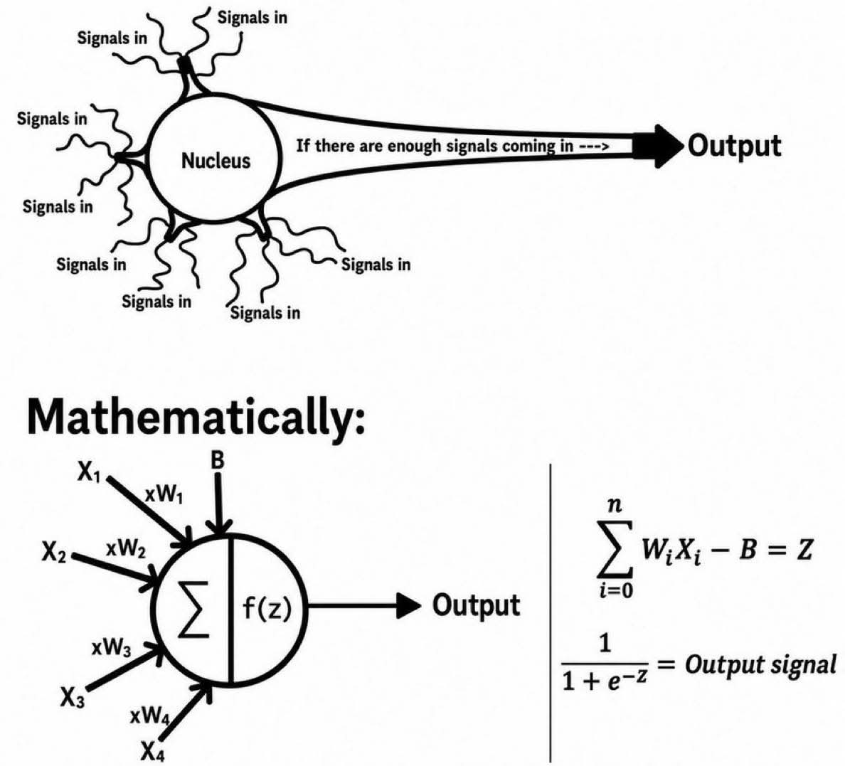
A biological neuron sums incoming signals and fires only if the total exceeds a threshold. The artificial neuron mimics this: inputs \(x_1,\dots,x_m\) carry weights \(w_1,\dots,w_m\), a bias \(b\) shifts the threshold, and the weighted sum \(z=w'x+b\) passes through an activation \(\psi(\cdot)\).

We use the logistic activation throughout \(\psi(z)=\frac{1}{1+e^{-z}}, \qquad \psi'(z)=\psi(z)\bigl(1-\psi(z)\bigr).\)

A Single Artificial Neuron

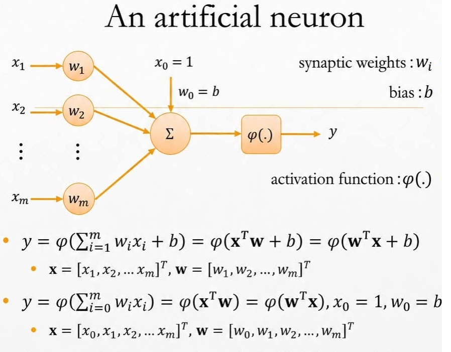
The neuron’s output is \(y = \psi(w'x+b) = \psi\!\Big(b + \sum_{i=1}^m w_i x_i\Big),\)

with inputs \(x=(x_1,\dots,x_m)'\), weights \(w=(w_1,\dots,w_m)'\), and bias \(b\). Absorbing the bias as \(w_0=b\), \(x_0=1\) gives the compact form \(y=\psi(\tilde{w}'\tilde{x})\).

A single logistic neuron is just a nonlinear regression function \(m(x;\theta)=\psi(w'x+b)\) with parameters \(\theta=(b,w')'\).

A Neuron Is an NLLS Model

Training the neuron by squared-error loss is exactly NLLS:

\[\hat{\theta} = \arg\min_{\theta}\sum_{i=1}^n \bigl(y_i-\psi(w'x_i+b)\bigr)^2.\]

Using \(\psi'=\psi(1-\psi)\), the gradient of \(m_i=\psi(z_i)\) with \(z_i=w'x_i+b\) is

\[\frac{\partial m_i}{\partial b}=\psi'(z_i), \qquad \frac{\partial m_i}{\partial w}=\psi'(z_i)\,x_i.\]

These rows form the Jacobian \(G(\theta)\). The FOCs \(G(\theta)'(y-m(X,\theta))=0\) are nonlinear, so the neuron is estimated by Gauss–Newton (the algorithm we saw in the previous chapter).

Single Hidden Layer Network: A Sum of Neurons

Stacking \(q\) logistic neurons and adding direct linear (“skip”) connections gives the augmented single-hidden-layer feedforward network:

\[m(x_i;\theta) = \underbrace{\alpha_0 + \alpha'x_i}_{\text{linear part}} + \sum_{j=1}^q \beta_j\,\psi\!\bigl(\gamma_{0j}+\gamma_j'x_i\bigr),\]

with \(\theta=(\alpha_0,\alpha',\{\beta_j,\gamma_{0j},\gamma_j'\}_{j=1}^q)'\) of dimension \(p=(1+k)+q(k+2)\).

• Setting \(\beta_1=\cdots=\beta_q=0\) recovers the linear model: OLS is nested.
• With enough hidden units \(q\), these functions are universal approximators of \(\mathbb{E}[y\mid x]\).

Estimation: Gauss–Newton \(\equiv\) Backpropagation

Let \(a_{ij}=\gamma_{0j}+\gamma_j'x_i\). The Jacobian rows of \(m(x_i;\theta)\) are

\[\frac{\partial m_i}{\partial \alpha_0}=1,\qquad \frac{\partial m_i}{\partial \alpha}=x_i,\qquad \frac{\partial m_i}{\partial \beta_j}=\psi(a_{ij}),\]

\[\frac{\partial m_i}{\partial \gamma_{0j}}=\beta_j\,\psi'(a_{ij}),\qquad \frac{\partial m_i}{\partial \gamma_j}=\beta_j\,\psi'(a_{ij})\,x_i.\]

These are exactly the quantities backpropagation computes by the chain rule.

• Gauss–Newton (second order): \(\theta^{(t+1)}=\theta^{(t)}+\bigl[G'G\bigr]^{-1}G'\bigl(y-m(X,\theta^{(t)})\bigr)\) — each step is an OLS regression of residuals on the Jacobian.
• Backpropagation is gradient descent (first order) on \(S(\theta)\): \(\theta^{(t+1)}=\theta^{(t)}+\eta\,G(\theta^{(t)})'\bigl(y-m(X,\theta^{(t)})\bigr)\).

From Gauss–Newton to Modern Machine Learning

A neural network is an NLLS estimator; what changes at scale is how we optimize and regularize.

• Scale. With millions of parameters, forming and inverting \(G'G\) is infeasible, so ML uses first-order methods (SGD, Adam) instead of Gauss–Newton.
• Regularization. A weight-decay penalty \(\lambda\bigl(\lVert\beta\rVert^2+\lVert\gamma\rVert^2\bigr)\) added to \(S(\theta)\) is exactly ridge shrinkage — it controls complexity and overfitting.
• Evaluation. Models are selected by out-of-sample prediction (cross-validation), not classical \(t\)/\(F\) inference.

Identification caveat. Under \(H_0:\beta_j=0\) the hidden weights \(\gamma_j\) drop out and are not identified; the standard \(t\) and \(\chi^2\) distributions fail, and simulation/bootstrap critical values are required.

3. Ridge and LASSO

(penalized least squares for stability and variable selection)

Why Penalization?

OLS behaves poorly when:

• Regressors are highly collinear — \((X'X)\) is nearly singular, estimates are unstable.
• The number of covariates is large relative to \(n\) — overfitting, poor out-of-sample performance.

The key idea: keep the linear predictor \(y_i \approx x_i'\beta\), but add a penalty that shrinks coefficients toward zero.

This introduces bias but drastically reduces variance — the classic bias–variance tradeoff.

Two approaches depending on the penalty function:

Method	Penalty	Variable Selection?
Ridge	\(\sum_j \beta_j^2\) (\(L_2\))	No — smooth shrinkage
LASSO	\(\sum_j |\beta_j|\) (\(L_1\))	Yes — exact zeros

Ridge Regression

Ridge solves

\[\hat{\beta}_{Ridge} = \arg\min_{\beta} \left\{\frac{1}{n}\sum_{i=1}^n (y_i-x_i'\beta)^2 + \lambda\sum_{j=1}^p \beta_j^2\right\}.\]

The quadratic penalty yields a closed-form solution:

\[\hat{\beta}_{Ridge} = (X'X + n\lambda I_p)^{-1}X'y.\]

Orthogonal design (\(X'X/n=I_p\)): each coefficient shrinks by the same factor,

\[\hat{\beta}_{j,Ridge} = \frac{1}{1+\lambda}\,\hat{\beta}_{j,OLS}.\]

• When \(\lambda=0\): reduces to OLS.
• As \(\lambda\uparrow\): all coefficients are pulled toward zero, but never exactly zero.

LASSO

LASSO solves

\[\hat{\beta}_{LASSO} = \arg\min_{\beta} \left\{\frac{1}{2n}\sum_{i=1}^n (y_i-x_i'\beta)^2 + \lambda\sum_{j=1}^p |\beta_j|\right\}.\]

The \(L_1\) penalty has a kink at zero — it can set coefficients exactly to zero: LASSO performs variable selection.

Orthogonal design — soft-thresholding solution:

\[\hat{\beta}_{j,LASSO} = \operatorname{sgn}(\hat{\beta}_{j,OLS})\max\!\left\{|\hat{\beta}_{j,OLS}|-\lambda,\;0\right\}.\]

• If \(|\hat{\beta}_{j,OLS}| \leq \lambda\): coefficient is set to exactly zero.
• If \(|\hat{\beta}_{j,OLS}| > \lambda\): coefficient survives but is shrunk by \(\lambda\).

Elastic Net

When regressors are highly correlated, LASSO arbitrarily picks one and drops others. Ridge shrinks correlated variables together but does not select.

The Elastic Net combines both penalties:

\[\hat{\beta}_{ElasticNet} = \arg\min_{\beta}\left\{\frac{1}{2n}\sum_{i=1}^n (y_i-x_i'\beta)^2 + \lambda\sum_{j=1}^p\!\left(\alpha|\beta_j| + \frac{1-\alpha}{2}\beta_j^2\right)\right\},\]

where \(\alpha\in[0,1]\) controls the mix:

• \(\alpha=1\): pure LASSO.
• \(\alpha=0\): pure Ridge.

Elastic Net produces sparse models like LASSO while maintaining the grouping effect of Ridge for correlated variables.

Bias–Variance Tradeoff and Tuning

The tuning parameter \(\lambda\) governs the bias–variance tradeoff:

• Small \(\lambda\) → little shrinkage → close to OLS (low bias, high variance).
• Large \(\lambda\) → strong shrinkage → low variance, higher bias.

Choosing \(\lambda\): not by hypothesis testing, but by \(K\)-fold cross-validation.

1. Partition the sample into \(K\) subsets.
2. Train on \(K-1\) subsets; evaluate on the held-out fold.
3. Select the \(\lambda\) (and \(\alpha\) for Elastic Net) that minimizes out-of-sample MSE.

Asymptotic comments (fixed-dimensional case):

• Ridge: consistent if \(\lambda_n\to 0\) at an appropriate rate.
• LASSO: consistent for prediction and estimation under suitable rates; variable-selection consistency requires stronger conditions.

Ridge and LASSO are still linear models — the fitted predictor remains linear in the covariates. What changes is the estimation criterion. They extend OLS, they do not replace it.

4. Quantile Regression

(modeling conditional quantiles beyond the conditional mean)

Why Move Beyond the Conditional Mean?

OLS targets \(\mathbb{E}[y_i\mid x_i]\) — the conditional mean.

But many questions concern other parts of the distribution:

• Do education programs help workers at the bottom of the wage distribution more than at the top?
• Does a policy variable affect downside risk differently from upside outcomes?

Quantile regression models conditional quantiles:

\[Q_{\tau}(y_i\mid x_i) = x_i'\beta(\tau), \qquad \tau\in(0,1).\]

Instead of one coefficient vector, we estimate a family \(\beta(\tau)\) indexed by the quantile level.

\(\beta_j(\tau)\) measures the marginal effect of \(x_{ij}\) on the \(\tau\)-th conditional quantile of \(y_i\). If \(\beta_j(\tau)\) varies with \(\tau\), effects are heterogeneous across the outcome distribution.

From LAD to the Check-Loss Function

Median (\(\tau=0.5\)): instead of minimizing squared residuals (OLS), minimize absolute residuals — Least Absolute Deviations (LAD):

\[\hat{\beta}_{LAD} = \arg\min_{\beta}\sum_{i=1}^n |y_i - x_i'\beta|.\]

LAD is more robust to outliers because it penalizes errors linearly, not quadratically.

General \(\tau\): replace the absolute value with the asymmetric check-loss function:

\[\rho_{\tau}(u) = u\bigl(\tau - \mathbf{1}\{u<0\}\bigr) = \begin{cases}\tau u, & u\geq 0,\\ (\tau-1)u, & u<0.\end{cases}\]

The quantile-regression estimator solves:

\[\hat{\beta}(\tau) = \arg\min_{\beta}\sum_{i=1}^n \rho_{\tau}(y_i-x_i'\beta).\]

Intuition Behind the Check-Loss

Why does asymmetric loss target quantiles?

Consider \(\tau=0.90\):

• Under-predictions (\(u\geq 0\)): penalized by factor \(0.90\) — heavily penalized.
• Over-predictions (\(u<0\)): penalized by factor \(0.10\) — lightly penalized.

This asymmetry forces the fitted line upward until 90% of observations lie below and 10% lie above — targeting the 90th conditional quantile.

First-order conditions (in subgradient form, since \(\rho_\tau\) is not everywhere differentiable):

\[\sum_{i=1}^n x_i\bigl(\tau - \mathbf{1}\{y_i - x_i'\beta < 0\}\bigr) = 0.\]

At the optimum, the weighted balance of positive and negative residuals is zero.

Asymptotic Normality of QR

Let \(Q_{\tau}(y_i\mid x_i)=x_i'\beta_0(\tau)\). Under standard regularity conditions:

\[\sqrt{n}\bigl(\hat{\beta}(\tau)-\beta_0(\tau)\bigr)\xrightarrow{\,d\,} \mathcal{N}(0,\,V_{\tau}),\]

where

\[V_{\tau} = \tau(1-\tau)\,D_{\tau}^{-1}\,Q\,D_{\tau}^{-1},\]

with

\[Q = \mathbb{E}[x_i x_i'], \qquad D_{\tau} = \mathbb{E}\bigl[f_{u_{\tau}\mid x}(0\mid x_i)\,x_i x_i'\bigr].\]

The term \(f_{u_\tau\mid x}(0\mid x_i)\) is the conditional density of the regression residual evaluated at zero.

Note: Unlike OLS, the asymptotic variance of QR depends on the conditional density at the quantile of interest — not just second moments of the regressors. Standard OLS variance formulas do not apply.

Summary: Extensions of OLS

Method	Relaxes	Keeps	Key Feature
GLS/FGLS	Homoskedasticity + independence	Linear conditional mean	Efficient under nonspherical errors
NLLS	Linearity in parameters	Least-squares criterion	Nonlinear regression functions
Ridge	OLS objective	Linear predictor	Smooth shrinkage, no selection
LASSO	OLS objective	Linear predictor	Shrinkage + variable selection
Quantile Reg.	Focus on conditional mean	Linear index	Effects at any quantile \(\tau\)

The common lesson: the linear model is not abandoned — it is adapted. Each extension keeps the core intuition of OLS while responding to a specific empirical challenge.

Cierre

¿Preguntas?

\[\,\]

O vía E-mail:
luis.chanci@usach.cl
luischanci@santotomas.cl