Maximum Likelihood Estimation (MLE)
Magíster en Economía
Teoría Econométrica (Econometric Theory)
Outline
- From OLS to MLE
- Likelihood, log-likelihood, score, and information
- Three canonical examples
- Asymptotic theory of MLE
- Efficiency, invariance, and inference
- Looking ahead: limited dependent variable models
Main idea: MLE chooses the parameter vector that makes the observed sample look most plausible under a specified probabilistic model.
1. From OLS to MLE
Why Another Estimation Method?
In OLS, we estimate parameters by minimizing a quadratic loss: \[ \hat\beta_{OLS} = \operatorname*{arg\,min}_\beta (y-X\beta)'(y-X\beta). \]
MLE also solves an optimization problem, but from a different angle:
Instead of minimizing a loss, MLE chooses the parameter vector that makes the observed sample most likely under a fully specified probability model.
This makes MLE both:
- an estimation method
- a modeling framework
Connection with OLS
There is a direct bridge from OLS to MLE.
In the Gaussian linear regression model, \[ y\mid X \sim \mathcal{N}(X\beta,\sigma^2 I_n), \] the MLE for \(\beta\) is exactly \[ \hat\beta_{MLE}=\hat\beta_{OLS}. \]
So OLS is not outside the likelihood framework. It is a special case of MLE under normal disturbances.
This is one reason MLE is a natural continuation of the OLS chapter.
Strengths and Cost of MLE
Relative to OLS or GMM, MLE has a clear advantage:
- it often delivers estimators with strong large-sample properties
- it gives a unified framework for estimation and inference
- it is the natural tool in many nonlinear models
But there is also a cost:
MLE requires stronger structure because we must specify a probability model for the data.
That is, we move from moment conditions to a full density or probability mass function.
2. The Likelihood Framework
The MLE Workflow
A single recipe runs through this whole chapter; every model below is just this pipeline applied to a different density:
model \(\;\rightarrow\;\) likelihood \(\mathcal{L}_n(\theta)\) \(\;\rightarrow\;\) log-likelihood \(\ell_n(\theta)\) \(\;\rightarrow\;\) score / Hessian \(s_n,\,H_n\) \(\;\rightarrow\;\) optimizer (closed form or Newton–Raphson) \(\;\rightarrow\;\) standard errors & tests (Wald / LR / Score)
Keep this map in mind: the algebra changes from model to model, but the steps never do.
From Probability to Likelihood
Suppose we observe \(\{w_i\}_{i=1}^n\), where each \(w_i\) has density or pmf \[ f(w_i;\theta), \qquad \theta\in\Theta\subset\mathbb{R}^k. \]
If the observations are independent and identically distributed (i.i.d.), the joint density factors as \[ f(w_1,\ldots,w_n;\theta)=\prod_{i=1}^n f(w_i;\theta). \]
Definition — Likelihood Function
Given the observed sample, the likelihood function is \(\mathcal{L}_n(\theta)=\prod_{i=1}^n f(w_i;\theta)\).
Holding the data fixed, we read this same expression as a function of \(\theta\): that is the likelihood.
The likelihood is not a probability over \(\theta\): it does not integrate to one, and it makes no probability statement about \(\theta\). It only ranks parameter values by how plausible they make the observed data.
The Maximum Likelihood Estimator
Definition — MLE
The Maximum Likelihood Estimator is \[ \hat\theta_{MLE} = \operatorname*{arg\,max}_{\theta\in\Theta}\mathcal{L}_n(\theta). \]
Intuition: among all parameter values, choose the one under which the observed sample looks most plausible.
Different values of \(\theta\) imply different probability models for the data. MLE picks the best-fitting one.
Why Use the Log-Likelihood?
In practice, we maximize \[ \ell_n(\theta)=\ln \mathcal{L}_n(\theta) = \sum_{i=1}^n \ln f(w_i;\theta). \]
Why?
- the logarithm is strictly increasing, so the maximizer does not change
- products become sums
- derivatives and numerical optimization become much easier
MLE
Therefore, using the log-likelihood, a more practical definition is
Definition
\[ \hat\theta_{MLE} = \operatorname*{arg\,max}_{\theta\in\Theta}\ell_n(\theta). \]
Notation: a subscript \(i\) is a per-observation quantity; a subscript \(n\) is its sum over the sample (\(\ell_n=\sum_i\ell_i\), and likewise for the score and Hessian below).
Score, Hessian, and Fisher Information
Definition — Score and Hessian
The score is the gradient of the log-likelihood: \[ s_n(\theta) = \frac{\partial \ell_n(\theta)}{\partial \theta} = \sum_{i=1}^n s_i(\theta). \]
The Hessian is the matrix of second derivatives: \[ H_n(\theta) = \frac{\partial^2 \ell_n(\theta)}{\partial \theta\,\partial \theta'} = \sum_{i=1}^n H_i(\theta). \]
At an interior optimum: \(s_n(\hat\theta)=0\). This is the likelihood analogue of the OLS normal equations.
Fisher Information
Definition — Fisher Information
The Fisher information in one observation is \[ \mathcal{I}(\theta)=\mathbb{E}[s_i(\theta)s_i(\theta)']. \]
Under standard regularity conditions, \[ \mathcal{I}(\theta) = -\mathbb{E}[H_i(\theta)]. \]
Sharp curvature of the log-likelihood \(\Rightarrow\) informative data \(\Rightarrow\) precise estimator. A flat likelihood \(\Rightarrow\) little information.
For an i.i.d. sample the information adds up: \(\mathcal{I}_n(\theta)=n\,\mathcal{I}(\theta)\) (this is why the sample tests below carry a factor of \(n\)).
Computing the MLE: Newton–Raphson
Most score equations \(s_n(\theta)=0\) are nonlinear and have no closed form (e.g. logit, below). We iterate:
\[ \theta^{(m+1)} = \theta^{(m)} - H_n\bigl(\theta^{(m)}\bigr)^{-1}\,s_n\bigl(\theta^{(m)}\bigr). \]
- direction from the score, rescaled by curvature (the Hessian)
- use step-halving / line search if a step lowers \(\ell_n\)
- diagnostics: \(\|s_n(\hat\theta)\|\approx 0\), \(H_n(\hat\theta)\) negative definite, stable across starting values
The Gaussian examples solve in closed form; everything beyond them is typically optimized numerically.
3. Canonical Examples
Example 1: Mean of a Normal (known variance \(\sigma^2=1\))
Suppose \[ z_i \overset{\text{i.i.d.}}{\sim} \mathcal{N}(\mu,1), \qquad i=1,\ldots,n, \] with the variance known and equal to 1, so the only unknown is \(\mu\).
The density is \[ f(z_i;\mu) = \frac{1}{\sqrt{2\pi}} \exp\left\{-\frac{(z_i-\mu)^2}{2}\right\}. \]
Hence the log-likelihood is \[ \ell_n(\mu) = -\frac{n}{2}\ln(2\pi) -\frac{1}{2}\sum_{i=1}^n (z_i-\mu)^2, \] and the score is \[ s_n(\mu)=\sum_{i=1}^n (z_i-\mu). \]
Example 1: Solving the FOC
Set the score equal to zero: \[ \sum_{i=1}^n (z_i-\hat\mu)=0 \quad\Longrightarrow\quad \hat\mu_{MLE}=\bar z. \]
The Hessian is \(H_n(\mu)=-n<0\), so the log-likelihood is globally concave and the FOC gives the global maximum. The information in one observation is \(\mathcal{I}(\mu)=1\), so \(\mathbb{V}(\hat\mu_{MLE})\approx 1/n\).
This simple example already shows the full MLE logic:
specify a density \(\rightarrow\) write the log-likelihood \(\rightarrow\) compute the score \(\rightarrow\) solve the FOC \(\rightarrow\) read precision from the curvature.
Example 2: The Normal Linear Regression Model
Now consider \[ y = X\beta + u, \qquad u\mid X \sim \mathcal{N}(0,\sigma^2 I_n). \]
Then \[ y\mid X \sim \mathcal{N}(X\beta,\sigma^2 I_n), \] and the log-likelihood is \[ \ell_n(\beta,\sigma^2) = -\frac{n}{2}\ln(2\pi) -\frac{n}{2}\ln(\sigma^2) -\frac{1}{2\sigma^2}(y-X\beta)'(y-X\beta). \]
For fixed \(\sigma^2\), maximizing the log-likelihood with respect to \(\beta\) is equivalent to minimizing the sum of squared residuals.
Example 2: MLE and OLS Coincide
Differentiate with respect to \(\beta\): \[ \frac{\partial \ell_n(\beta,\sigma^2)}{\partial \beta} = \frac{1}{\sigma^2}X'(y-X\beta). \]
Set equal to zero: \[ X'X\hat\beta=X'y. \]
Therefore, \[ \hat\beta_{MLE}=(X'X)^{-1}X'y=\hat\beta_{OLS}. \]
For the variance parameter, \[ \hat\sigma^2_{MLE} = \frac{(y-X\hat\beta)'(y-X\hat\beta)}{n}. \]
This divides by \(n\), not \(n-k\): the MLE maximizes likelihood, not finite-sample unbiasedness. The bias is \(O(k/n)\) and vanishes asymptotically.
Example 3: A Discrete Model — Bernoulli
Why do we need MLE beyond least squares? Take a binary outcome \[ y_i \overset{\text{i.i.d.}}{\sim} \mathrm{Bernoulli}(p), \qquad f(y_i;p)=p^{y_i}(1-p)^{1-y_i}. \]
Log-likelihood and score: \[ \ell_n(p)=\sum_{i=1}^n\bigl[y_i\ln p+(1-y_i)\ln(1-p)\bigr], \qquad s_n(p)=\frac{\sum_i y_i-np}{p(1-p)}. \]
FOC \(\Rightarrow \hat p_{MLE}=\bar y\). The information is \(\mathcal{I}(p)=\dfrac{1}{p(1-p)}\), so \(\mathbb{V}(\hat p)\approx p(1-p)/n\).
Information is largest near \(p=0\) or \(p=1\) and smallest at \(p=\tfrac12\): boundary outcomes are the most informative.
From Bernoulli to Logistic Regression
Let the success probability depend on covariates through the logistic link: \[ \Pr(y_i=1\mid x_i)=\Lambda(x_i'\beta), \qquad \Lambda(a)=\frac{1}{1+e^{-a}}. \]
Using \(\Lambda'=\Lambda(1-\Lambda)\), the score is \[ s_n(\beta)=\sum_{i=1}^n\bigl(y_i-\Lambda(x_i'\beta)\bigr)x_i. \]
No closed form \(\Rightarrow\) solve by Newton–Raphson. This is the prototype for the logit/probit models in Section 6, and the clearest case where MLE, not OLS, is the default.
4. Asymptotic Theory of MLE
Regularity Conditions: Big Picture
For MLE asymptotics, we need:
- correct specification of the model
- identification of the true parameter
- smoothness of the log-likelihood
- nonsingularity of the information matrix
- LLN and CLT conditions for the score and Hessian
Regularity conditions for MLE
These conditions ensure that the expected log-likelihood is uniquely maximized at \(\theta_0\) and that derivatives behave well enough for Taylor expansions and probabilistic limits.
Consistency of MLE
Let \[ Q_n(\theta)=\frac{1}{n}\ell_n(\theta). \]
Under a suitable (uniform) LLN, \[ Q_n(\theta)\xrightarrow{p} Q(\theta)=\mathbb{E}[\ell_i(\theta)]. \]
If the population criterion \(Q(\theta)\) is uniquely maximized at \(\theta_0\) (identification), then the maximizer of the sample criterion converges to it: \[ \hat\theta_{MLE}\xrightarrow{p} \theta_0. \]
Consistency of MLE
Consistency of MLE
Under standard regularity conditions, \[ \hat\theta_{MLE}\xrightarrow{\,p\,}\theta_0. \]
MLE is an extremum estimator: consistency comes from the sample criterion converging to a population criterion with a unique maximizer.
Asymptotic Normality: Step 1
The score satisfies \[ s_n(\hat\theta)=0. \]
Expand around \(\theta_0\): \[ 0 = s_n(\theta_0) + H_n(\tilde\theta)(\hat\theta-\theta_0), \] where \(\tilde\theta\) lies between \(\hat\theta\) and \(\theta_0\).
Rearranging, \[ \sqrt{n}(\hat\theta-\theta_0) = - \left[\frac{1}{n}H_n(\tilde\theta)\right]^{-1} \left[\frac{1}{\sqrt{n}}s_n(\theta_0)\right]. \]
This isolates the two key objects: the score and the Hessian.
Asymptotic Normality: Step 2
The score is a sum of i.i.d. terms, \[ s_n(\theta_0)=\sum_{i=1}^n s_i(\theta_0), \qquad \mathbb{E}[s_i(\theta_0)]=0, \] so the CLT gives \[ \frac{1}{\sqrt{n}}s_n(\theta_0) \xrightarrow{d} \mathcal{N}(0,\mathcal{I}(\theta_0)). \]
Since \(\hat\theta\xrightarrow{p}\theta_0\), also \(\tilde\theta\xrightarrow{p}\theta_0\), and by the LLN (with the information equality) \[ -\frac{1}{n}H_n(\tilde\theta)\xrightarrow{p} \mathcal{I}(\theta_0). \]
Asymptotic Normality: Final Result
By Slutsky’s theorem, \[ \sqrt{n}(\hat\theta_{MLE}-\theta_0) \xrightarrow{d} \mathcal{N}\bigl(0,\mathcal{I}(\theta_0)^{-1}\bigr). \]
Asymptotic normality of MLE
Under standard regularity conditions, \[ \sqrt{n}(\hat\theta_{MLE}-\theta_0) \xrightarrow{d} \mathcal{N}\bigl(0,\mathcal{I}(\theta_0)^{-1}\bigr). \]
Foundation for standard errors, confidence intervals, and large-sample tests. Sharp curvature (large \(\mathcal{I}\)) \(\Rightarrow\) small variance.
Variance Estimation in Practice
The asymptotic variance depends on the unknown information matrix, so we estimate it (all at \(\hat\theta\)):
- Observed information
\[\widehat{\operatorname{Var}}_H(\hat\theta) = [-H_n(\hat\theta)]^{-1} \] - Outer product of gradients (OPG) \[\widehat{\operatorname{Var}}_{OPG}(\hat\theta) = \left(\sum_{i=1}^n s_i(\hat\theta)s_i(\hat\theta)'\right)^{-1} \] - Sandwich form (robust / QMLE) \[\widehat{\operatorname{Var}}_{sand}(\hat\theta) = \frac{1}{n}A_n^{-1}B_nA_n^{-1} \]
where \(A_n=-\tfrac{1}{n}H_n(\hat\theta)\) and \(B_n=\tfrac{1}{n}\sum_i s_i(\hat\theta)s_i(\hat\theta)'\).
Correct specification \(\Rightarrow\) all three coincide (\(A_n=B_n=\mathcal{I}\)). Misspecification (QMLE) \(\Rightarrow\) use the sandwich \(A_n^{-1}B_nA_n^{-1}\).
5. Efficiency, Invariance, and Inference
The Cramér–Rao Lower Bound
For an unbiased scalar estimator \(\tilde\theta\), \[ \mathbb{V}(\tilde\theta)\geq \frac{1}{\mathcal{I}_n(\theta_0)}, \qquad \mathcal{I}_n(\theta_0)=n\mathcal{I}(\theta_0). \]
Intuition: the more sharply the likelihood responds to changes in \(\theta\), the more informative the data, and the smaller the lower bound on variance.
Why MLE Is Called Efficient
MLE is not necessarily unbiased in finite samples, so the finite-sample Cramér–Rao result must be read carefully.
What is true is that, under correct specification, \[ \sqrt{n}(\hat\theta_{MLE}-\theta_0) \xrightarrow{d} \mathcal{N}(0,\mathcal{I}(\theta_0)^{-1}), \] and no regular estimator has a smaller asymptotic covariance.
Asymptotic efficiency of MLE
Under correct specification and standard regularity conditions, MLE attains the asymptotic information bound \(\mathcal{I}(\theta_0)^{-1}\), i.e., it is asymptotically efficient among regular estimators.
The Invariance Property
Invariance of MLE
If \(\gamma=g(\theta)\) for a continuous one-to-one \(g(\cdot)\) and \(\hat\theta_{MLE}\) is the MLE of \(\theta\), then \[ \hat\gamma_{MLE}=g(\hat\theta_{MLE}). \]
Example: if the MLE of \(\sigma^2\) is \(\hat\sigma^2_{MLE}\), then the MLE of \(\sigma\) is simply \[ \hat\sigma_{MLE}=\sqrt{\hat\sigma^2_{MLE}}. \]
No new optimization is needed for a smooth transformation of the parameters (handy for elasticities, marginal effects, odds ratios).
Wald Tests
Suppose \[ H_0:R\theta=r. \]
The Wald statistic is \[ W = (R\hat\theta-r)' \bigl[ R\widehat{\operatorname{Var}}(\hat\theta)R' \bigr]^{-1} (R\hat\theta-r) \xrightarrow{d} \chi_q^2 \;\text{ under } H_0. \]
The Wald test asks whether the unrestricted estimate lies far from the null restriction once that distance is scaled by estimation uncertainty. It needs only the unrestricted fit.
Likelihood Ratio and Score Tests
Let \(\hat\theta_u\) be the unrestricted MLE and \(\tilde\theta_r\) the restricted MLE.
Likelihood Ratio test (needs both fits) \[ LR = 2\bigl[\ell_n(\hat\theta_u)-\ell_n(\tilde\theta_r)\bigr] \xrightarrow{d} \chi_q^2. \]
Score / LM test (needs only the restricted fit) \[ LM = s_n(\tilde\theta_r)' \bigl[n\widehat{\mathcal{I}}(\tilde\theta_r)\bigr]^{-1} s_n(\tilde\theta_r) \xrightarrow{d} \chi_q^2. \]
All three are asymptotically \(\chi_q^2\) and locally equivalent under \(H_0\) (\(W-LR=o_p(1)\), \(LR-LM=o_p(1)\)); they differ in how much estimation they require.
Geometric Intuition: Wald vs. LR
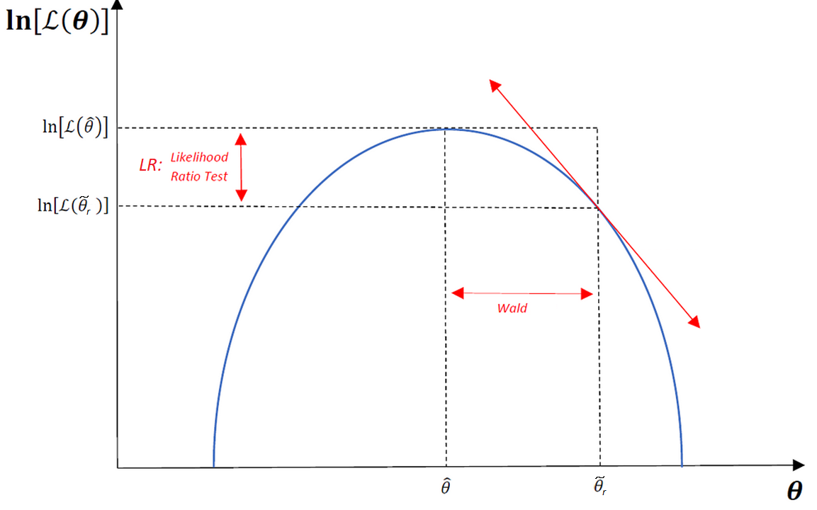
- Wald: how far the unrestricted estimate is from the null set (distance)
- LR: how much the fit worsens when the restriction is imposed (gap in fit)
- Score: how steep the log-likelihood still is at the restricted estimate (slope)
6. Looking Ahead
MLE as a Unifying Framework
- OLS \(=\) Gaussian MLE of \(\beta\) under homoskedastic normal errors; \(\hat\sigma^2_{MLE}\) divides by \(n\)
- GLS \(=\) Gaussian MLE of \(\beta\) under \(u\mid X\sim\mathcal{N}(0,\sigma^2\Omega)\)
- Logit / Probit \(=\) MLE for binary outcomes (Bernoulli likelihood)
Only the assumed density changes from one model to the next; the estimation and inference machinery is identical.
Why MLE Matters Beyond Gaussian Regression
The real power of MLE appears when OLS is no longer natural.
Examples:
- binary outcomes \(\rightarrow\) logit and probit
- unordered / ordered choices \(\rightarrow\) multinomial and ordered models
- count outcomes \(\rightarrow\) Poisson (\(\lambda=\exp(X\beta)\))
- censored / selected outcomes \(\rightarrow\) Tobit, Heckman
- duration data \(\rightarrow\) hazard / survival models
The logic remains the same: specify a probabilistic model, write the likelihood, optimize it (usually by Newton–Raphson), and use information-based asymptotic theory for inference.
Summary
MLE chooses the parameter vector that makes the observed sample most plausible under a specified probability model.
The score, Hessian, and Fisher information organize both estimation and inference; Newton–Raphson computes the estimator when no closed form exists.
In the Gaussian linear model, MLE coincides with OLS; the Bernoulli/logit model shows why MLE is needed beyond least squares.
Under standard regularity conditions, \[ \sqrt{n}(\hat\theta_{MLE}-\theta_0) \xrightarrow{d} \mathcal{N}\bigl(0,\mathcal{I}(\theta_0)^{-1}\bigr). \]
Wald, LR, and Score tests emerge naturally and are asymptotically equivalent under \(H_0\).
Cierre

\[\,\]
luis.chanci@usach.cl
luischanci@santotomas.cl