Instrumental Variables (IV) and 2SLS

Magíster en Economía
Teoría Econométrica (Econometric Theory)

Prof. Luis Chancí

www.luischanci.com

Outline

Endogeneity and why OLS fails
Instrument validity: relevance, exogeneity, exclusion (+ finding instruments)
The exactly identified scalar case (reduced form / first stage / IV ratio)
LATE and the interpretation of IV
Two-Stage Least Squares (2SLS)
Asymptotic theory and inference
Diagnostics: weak instruments, overidentification, exogeneity
Applied example: returns to schooling in R (and Stata)
Bridge to GMM

Main idea: when a regressor is correlated with the error, OLS is inconsistent. IV replaces the contaminated variation in the regressor with exogenous variation supplied by an instrument.

1. Endogeneity and Why OLS Fails

When Does OLS Break Down?

Consider \[ y_i=x_i'\beta+u_i. \]

If \(\mathbb{E}[x_i u_i]=0\), OLS is consistent.
If \(\mathbb{E}[x_i u_i]\neq 0\) (endogeneity), OLS is generally inconsistent.

Endogeneity: the regressor carries variation systematically related to the unobserved determinants of \(y\). The OLS coefficient then mixes the structural effect with spurious correlation.

A Running Empirical Example: Returns to Schooling

A concrete face for the error term makes the algebra easier to read. Consider the classic returns-to-schooling question (Card, 1995): \[ \log(\text{wage})_i=\beta_0+\beta_1\,\text{schooling}_i+u_i. \]

Ability bias. Unobserved ability, family background, motivation, and networks sit inside \(u_i\) and also raise schooling. So \(\mathbb{E}[\text{schooling}_i\,u_i]\neq 0\), and the OLS return \(\hat\beta_1\) blends the causal return with selection.

We cannot randomly assign schooling. IV looks instead for a variable that shifts schooling but is unrelated to ability — e.g. proximity to a college (Card) or parental education.

Sources of Endogeneity

Omitted variables: a determinant of \(y\) is left out and correlated with \(x\) (e.g. ability)
Simultaneity / reverse causality: \(x\) and \(y\) are jointly determined (e.g. price and quantity)
Measurement error: \(x\) is observed with error
Sample selection, dynamic panel bias: further common cases

For the omitted-variable case, the short regression gives \[ \operatorname{plim}\hat\beta_1^{OLS} = \beta_1+\beta_2\frac{\operatorname{Cov}(x_1,x_2)}{\operatorname{Var}(x_1)}. \]

The bias vanishes only if \(\beta_2=0\) or \(\operatorname{Cov}(x_1,x_2)=0\).

DAG Intuition

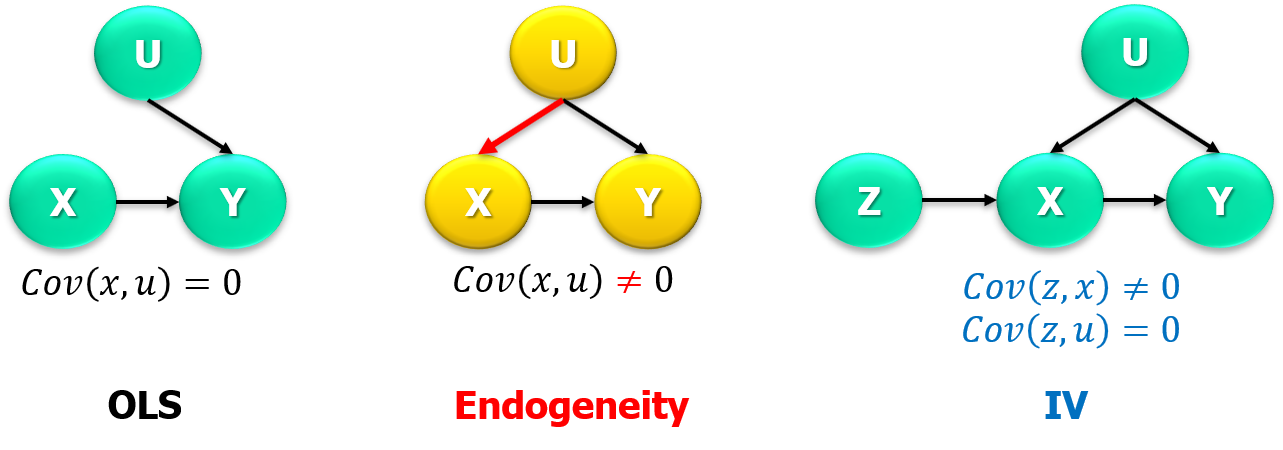
Left: \(X\) exogenous — OLS is fine.
Middle: \(U\) affects both \(X\) and \(Y\) — a back-door path makes \(X\) endogenous.
Right: instrument \(Z\) moves \(X\) but has no path to \(U\) — IV uses this variation.

From the DAG to Moment Conditions

The two arrows that define a valid instrument translate directly into two moments:

Relevance (\(Z\to X\)): \(\operatorname{Cov}(Z,X)\neq 0\).
Exclusion / exogeneity (\(Z\) reaches \(Y\) only through \(X\), and \(U\not\to Z\)): \(\mathbb{E}[Z\,u]=0\).

The whole IV method is the statement that these two moments are enough to recover \(\beta\) — provided the second one truly holds.

Instrument Validity Is Two Claims, Not One

In DAG language, a valid instrument requires two distinct things:

Relevance: an open path from \(z_i\) to \(x_i\) (\(z\) moves \(x\))
Exclusion / exogeneity: every path from \(z_i\) to \(y_i\) other than through \(x_i\) is blocked

Relevance can be checked in the data. Exclusion/exogeneity cannot be verified from data alone — it must be defended with economic theory, institutions, or design. In applied work, this is the hard one.

2. Conditions for a Valid Instrument

The Three Informal Conditions

Relevance: the instrument is related to the endogenous regressor
Exogeneity: the instrument is orthogonal to the structural error
Exclusion: the instrument affects \(y\) only through the endogenous regressor

Exclusion is usually the key economic assumption: it rules out any direct channel from the instrument to the outcome.

The Instrument’s “Story” (Schooling Example)

The conditions are not just algebra — each needs a narrative:

Relevance — why \(Z\) moves schooling? Proximity to a college lowers the cost of attending; parental education shapes expectations and resources. Both plausibly raise years of schooling.
Exclusion — why \(Z\) is absent from the wage equation? This is contestable. Does growing up near a college, or having educated parents, affect wages only through your own schooling?

For parental education, exclusion is doubtful: educated parents may transmit ability, networks, and preferences that affect wages directly. We keep the example precisely because it is intuitive but not perfectly clean.

Formal Conditions

For \(y_i=x_i'\beta+u_i\) with an \(r\times1\) instrument vector \(z_i\):

Instrument validity

Exogeneity: \(\mathbb{E}[z_i u_i]=0\)
Relevance: \(\operatorname{rank}\bigl(\mathbb{E}[z_i x_i']\bigr)=k\)

Relevance is a rank condition, not a set of pairwise correlations: the instruments must generate enough independent variation to identify all \(k\) parameters jointly.

Order vs. Rank Condition

Two conditions students often confuse

Order condition (necessary): at least as many instruments as endogenous regressors, \(r\ge k\) — a counting rule.
Rank condition (necessary and sufficient): \(\mathbb{E}[z_i x_i']\) has full column rank \(k\) — the instruments are actually informative, so the relevant matrices invert.

Passing the order condition without the rank condition = having “enough” instruments that are nonetheless uninformative.

A Hall of Fame of Instruments

Card (1995): proximity to a college \(\to\) years of schooling (returns to education).
Angrist (1990): Vietnam draft-lottery number \(\to\) military service (effect on earnings).
Angrist–Krueger (1991): quarter of birth \(\to\) schooling, via compulsory-schooling laws.
Parental education \(\to\) schooling — intuitive but exclusion is debatable.
Bartik / shift-share: national sectoral shocks \(\times\) local industry shares (regional labor demand).
Policy assignment / eligibility rules \(\to\) program take-up.

IV is not only an estimator; it is a research-design tool. The instruments above are arguments about where exogenous variation comes from.

Finding Instruments: A Checklist

Before trusting an instrument, as researcher we ask:

Does it create real variation in the endogenous regressor? (relevance)
Is the source of variation plausibly exogenous?
Can the exclusion restriction be defended institutionally?
Is the first stage strong enough (not weak)?
Are there multiple instruments, enabling overidentification tests?
Could it affect the outcome through another channel?

Sometimes a policy supplies variation directly; often the researcher must construct it (shift-share, simulated, or granular instruments).

Granular Instrumental Variables (GIV)

When no external shifter (a policy, a tax, geography) is available, the instrument can sometimes be built from inside the system itself. Gabaix and Koijen (JPE, 2024) show how (when a few players are very large).

Granular hypothesis. In heavy-tailed size distributions, idiosyncratic shocks to the largest players (Apple, a major bank, a giant asset manager) do not wash out. They are big enough to move aggregates, yet firm-specific enough to be unrelated to economy-wide shocks.

So an internal, idiosyncratic disturbance to a mega-player is relevant (it shifts the aggregate) and plausibly exogenous (it is unrelated to common macro shocks) — exactly the two things an instrument needs.

Constructing a Granular Instrument

Let firm \(i\)’s growth load on unobserved common shocks \(\eta_t\) plus an idiosyncratic part \(u_{it}\): \(\;y_{it}=\lambda_i\,\eta_t+u_{it}\). Compare two weighted averages of the same data:

Equal-weighted mean: idiosyncratic terms average out, so it tracks the common shock, \(\;\tfrac1N\sum_i y_{it}\approx \bar\lambda\,\eta_t\).
Size-weighted mean: dominated by the giants, so it keeps both \(\eta_t\) and their idiosyncratic shocks.

Subtracting one from the other purges the common component and isolates the granular residual: \[ Z_t=\sum_{i}\Bigl(S_{it}-\tfrac1N\Bigr)y_{it}\;\approx\;\sum_{i}\Bigl(S_{it}-\tfrac1N\Bigr)u_{it}, \] where \(S_{it}\) is firm \(i\)’s size share.

In practice: assemble a panel of the largest entities (funds, banks, firms), partial out estimated common factors, and build \(Z_t\) from the size-weighted idiosyncratic shocks (e.g. a huge fund rebalancing for internal reasons). The first stage regresses the aggregate endogenous variable on \(Z_t\) (relevant — the player is large enough to move the aggregate); 2SLS then recovers the structural elasticity, e.g. the demand elasticity of the stock market (Gabaix–Koijen’s “inelastic markets”).

Like a Bartik instrument, \(Z_t\) is constructed, not found — but the variation comes from large idiosyncratic shocks, not national sectoral trends. As always, validity hinges on exclusion: the giants’ idiosyncratic shocks must be uncorrelated with the common macro shocks.

3. The Exactly Identified Scalar Case

Covariance Derivation

Model \(y_i=\beta x_i+u_i\) with scalar instrument \(z_i\) and \(\mathbb{E}[z_iu_i]=0\).

Take covariances with \(z_i\): \[ \operatorname{Cov}(z_i,y_i)=\beta\,\operatorname{Cov}(z_i,x_i)+\underbrace{\operatorname{Cov}(z_i,u_i)}_{=0}. \]

So (with an intercept / demeaned variables) \[ \hat\beta_{IV} = \frac{\sum_i (z_i-\bar z)(y_i-\bar y)}{\sum_i (z_i-\bar z)(x_i-\bar x)}. \]

\(\beta\) is identified by how \(z\) co-moves with \(y\) relative to how \(z\) co-moves with \(x\).

Reduced Form ÷ First Stage

The scalar IV estimator is a ratio of two simple regressions — the most intuitive view for applied work:

First stage (\(z\to x\)): \(\quad x_i=\pi_0+\pi_1 z_i+v_i\)
Reduced form (\(z\to y\)): \(\quad y_i=\gamma_0+\gamma_1 z_i+\eta_i\)

\[ \hat\beta_{IV} = \frac{\widehat{\operatorname{Cov}}(z,y)}{\widehat{\operatorname{Cov}}(z,x)} = \frac{\hat\gamma_1}{\hat\pi_1} = \frac{\text{Reduced Form}}{\text{First Stage}}. \]

Read it as: “how much \(y\) moves with the instrument” divided by “how much \(x\) moves with the instrument.” We verify this numerically later in R.

Moment-Condition Derivation and a Number

From \(\mathbb{E}[z_i(y_i-x_i\beta)]=0\), the sample analogue gives \[ \hat\beta_{IV} = \Bigl(\textstyle\sum_i z_i x_i\Bigr)^{-1}\Bigl(\textstyle\sum_i z_i y_i\Bigr). \]

Example — scalar IV from sample covariances

If \(\widehat{\operatorname{Cov}}(z,y)=4\) and \(\widehat{\operatorname{Cov}}(z,x)=2\), then \[ \hat\beta_{IV}=\frac{4}{2}=2. \]

Only the part of \(x\) associated with \(z\) is used; the potentially contaminated part never enters.

4. LATE and the Interpretation of IV

IV Estimates Are Often a LATE

Theory often writes a single constant effect \(\beta\). With heterogeneous effects, 2SLS does not recover the average effect for everyone — it recovers a Local Average Treatment Effect (LATE): the effect for compliers, those whose treatment status responds to the instrument.

Recast the system with treatment \(D\) and instrument \(Z\):

Object	Equation	Interpretation
Structural	\(Y=\alpha+\delta D+\varepsilon\)	causal effect of \(D\) on \(Y\)
First stage	\(D=\pi_0+\pi_1 Z+\nu\)	instrument shifts treatment
Reduced form	\(Y=\gamma_0+\gamma_1 Z+\eta\)	instrument shifts outcome (ITT)
IV (LATE)	\(\delta=\gamma_1/\pi_1\)	effect for compliers

Compliers, ITT, and Monotonicity

ITT (reduced form \(\gamma_1\)): effect of being assigned/encouraged by the instrument, regardless of uptake.
First stage (\(\pi_1\)): how strongly assignment shifts actual treatment (compliance).
Wald / IV ratio \(\gamma_1/\pi_1\): scales the ITT up by the compliance rate \(\Rightarrow\) LATE.

Population types: compliers, always-takers, never-takers, defiers. The key identifying assumption is monotonicity: the instrument pushes everyone (weakly) in the same direction, i.e. no defiers.

So an IV estimate is causal for a specific margin of variation — the compliers induced by that instrument — not necessarily the ATE.

“IV Is Not Magic”

A reality check before the mechanics:

IV fixes endogeneity only if the instrument is valid.
A strong first stage does not guarantee exogeneity.
Overidentification tests do not prove instrument validity.
Weak instruments can make IV worse than OLS.
IV estimates may be local (LATE) to a particular margin.

5. Two-Stage Least Squares (2SLS)

Structural Model and Instruments

Partition \[ y_i=x_{1i}'\beta_1+x_{2i}'\beta_2+u_i, \]

\(x_{1i}\): \(m\times1\) endogenous regressors
\(x_{2i}\): \(p\times1\) included exogenous regressors

Instruments: \[ z_i=\begin{bmatrix} z_{1i}\\ x_{2i}\end{bmatrix}, \] where \(z_{1i}\) are excluded instruments and \(x_{2i}\) instrument themselves.

The 2SLS Estimator via \(P_Z\)

Define the projection matrix \[ P_Z=Z(Z'Z)^{-1}Z'. \]

Then \[ \hat\beta_{2SLS} = (X'P_Z X)^{-1}X'P_Z y = (\hat X'\hat X)^{-1}\hat X'y, \qquad \hat X=P_Z X. \]

\(\hat X=P_Z X\) are the first-stage fitted values, and 2SLS is just OLS of \(y\) on \(\hat X\) — which is why it is called Two-Stage Least Squares.

What the Two Stages Actually Do

First stage. Regress each endogenous regressor \(X_1\) on the full instrument set \(Z=[Z_1\;X_2]\): \[ \hat X_1=P_Z X_1. \] The exogenous \(X_2\) need no first stage (\(P_Z X_2=X_2\)): they instrument themselves.

Second stage. Regress \(y\) on \(\hat X_1\) and \(X_2\).

Only the endogenous regressors are replaced by fitted values; the exogenous regressors pass through unchanged. The compact \((X'P_ZX)^{-1}X'P_Zy\) works because \(X_2\in\text{col}(Z)\).

A Caution on Standard Errors

Why naive second-stage SEs are wrong

The manual second stage is a computational device, not the statistical model. OLS standard errors from regressing \(y\) on \(\hat X_1, X_2\) do not reproduce the sampling variance of 2SLS.

Use the 2SLS variance formula from the original equation — preferably the heteroskedasticity-robust version.

From Matrix Algebra to Software

The same point, shown in code: manual two-stage OLS reproduces the coefficient but reports the wrong standard error; ivreg() gives the correct one.

# Manual 2SLS (one endogenous regressor, one instrument)
fs       <- lm(schooling ~ educ_mom, data = wage_df)        # first stage
sch_hat  <- fitted(fs)
manual   <- lm(wage ~ sch_hat, data = wage_df)              # naive second stage
iv1      <- ivreg(wage ~ schooling | educ_mom, data = wage_df)

# Same point estimate, DIFFERENT (naive vs correct) standard error:
rbind(manual_OLS = coef(summary(manual))["sch_hat", 1:2],
      ivreg      = coef(summary(iv1))["schooling", 1:2])
#>            Estimate Std. Error
#> manual_OLS 108.2138   17.83964
#> ivreg      108.2138   18.02104

Lesson: the theoretical \(V_{IV}\) you derive is exactly what ivreg/ivregress implement. Never report manual second-stage OLS standard errors.

OLS as a Special Case

If all regressors are exogenous, take \(Z=X\), so \(P_Z=P_X\) and \[ \hat\beta_{2SLS} = (X'P_XX)^{-1}X'P_Xy = (X'X)^{-1}X'y = \hat\beta_{OLS}. \]

OLS is IV in which the regressors instrument themselves. IV extends OLS to endogenous regressors; with no endogeneity, they coincide.

6. Asymptotic Theory of IV

Regularity Conditions

Let \(Q_{ZX}=\mathbb{E}[z_ix_i']\), \(Q_{ZZ}=\mathbb{E}[z_iz_i']\).

Regularity conditions for IV

\(\{(y_i,x_i,z_i)\}\) i.i.d.
\(\mathbb{E}[z_iu_i]=0\)
\(Q_{ZZ}\) positive definite
\(\operatorname{rank}(Q_{ZX})=k\)
moment conditions for the LLN and CLT

Consistency

From \(\hat\beta_{2SLS}=\beta_0+(X'P_ZX)^{-1}X'P_Zu\) and the LLN: \[ \frac{X'Z}{n}\xrightarrow{\,p\,} Q_{XZ}, \quad \frac{Z'Z}{n}\xrightarrow{\,p\,} Q_{ZZ}, \quad \frac{Z'u}{n}\xrightarrow{\,p\,} \mathbb{E}[z_iu_i]=0. \]

Therefore \[ \hat\beta_{2SLS}\xrightarrow{\,p\,}\beta_0. \]

Exogeneity does the work: \(\frac{Z'u}{n}\xrightarrow{\,p\,} 0\) drives the estimation error to zero. The instruments isolate the part of \(X\) orthogonal to the error.

Asymptotic Normality

Write \(\sqrt{n}(\hat\beta_{2SLS}-\beta_0)=A_n^{-1}C_n\). Then \[ A_n\xrightarrow{\,p\,} A=Q_{XZ}Q_{ZZ}^{-1}Q_{ZX}, \qquad \frac{Z'u}{\sqrt n}\xrightarrow{\,d\,}\mathcal{N}(0,S), \quad S=\mathbb{E}[z_iz_i'u_i^2]. \]

By Slutsky, \[ \sqrt{n}(\hat\beta_{2SLS}-\beta_0)\xrightarrow{\,d\,}\mathcal{N}(0,V_{IV}), \quad V_{IV}=A^{-1}\bigl(Q_{XZ}Q_{ZZ}^{-1}S\,Q_{ZZ}^{-1}Q_{ZX}\bigr)A^{-1}. \]

We write the moment covariance as \(S\) (not \(\Omega\), reserved for GLS), to line up with the GMM notes.

Variance Estimation

Homoskedastic case (\(S=\sigma^2Q_{ZZ}\)): \[ \widehat{\operatorname{Var}}(\hat\beta_{2SLS})=\hat\sigma^2(X'P_ZX)^{-1}, \qquad \hat\sigma^2=\frac{\hat u'\hat u}{n-k},\;\;\hat u=y-X\hat\beta_{2SLS}. \]

Heteroskedasticity-robust: \[ \widehat{\operatorname{Var}}(\hat\beta_{2SLS})=\tfrac{1}{n}\hat A^{-1}\hat B\hat A^{-1}, \quad \hat S=\tfrac1n\textstyle\sum_i \hat u_i^2 z_iz_i'. \]

\(\hat u\) are structural residuals (original equation), not first-stage residuals. With time-series / panel / clustered data, replace \(\hat S\) by a HAC or cluster-robust estimator.

Robust Standard Errors in Practice

Why this matters empirically:

Homoskedastic 2SLS SEs rely on strong assumptions rarely met in micro data.
Default to heteroskedasticity-robust SEs; with clustered/panel data use cluster-robust inference.
Software lets you swap the variance estimator without changing the point estimate.

# Same IV point estimate, heteroskedasticity-robust (HC1) standard errors
lmtest::coeftest(iv1, vcov = sandwich::vcovHC, type = "HC1")
#> 
#> t test of coefficients:
#> 
#>             Estimate Std. Error t value  Pr(>|t|)    
#> (Intercept) -501.474    226.111 -2.2178   0.02688 *  
#> schooling    108.214     16.784  6.4475 2.083e-10 ***
#> ---
#> Signif. codes:  0 '***' 0.001 '**' 0.01 '*' 0.05 '.' 0.1 ' ' 1

In R: AER::ivreg() with sandwich::vcovHC, or estimatr::iv_robust() (robust by default). In Stata: ivregress 2sls ..., robust.

7. Diagnostics

Weak Instruments

If \(z\) is only weakly correlated with \(x\), 2SLS is biased and imprecise, and standard inference is distorted.

First-stage \(F\) rule of thumb

Single endogenous regressor, homoskedastic case (Staiger–Stock, 1997): the first-stage \(F\) on the excluded instruments should comfortably exceed 10.

Only a heuristic. With multiple endogenous regressors, heteroskedasticity, or clustering, use robust weak-instrument diagnostics (e.g. Kleibergen–Paap). Weak instruments pull 2SLS toward OLS and make its distribution non-normal.

First-Stage Diagnostic in Practice

Does the instrument actually predict schooling? Report the first-stage coefficient and the \(F\) on the excluded instruments.

fs1 <- lm(schooling ~ educ_mom, data = wage_df)            # one instrument
fs2 <- lm(schooling ~ educ_mom + educ_dad, data = wage_df) # two instruments

# First-stage F on the excluded instrument(s)
c(F_one_instrument  = summary(fs1)$fstatistic[["value"]],
  F_two_instruments = summary(fs2)$fstatistic[["value"]])
#>  F_one_instrument F_two_instruments 
#>         115.46720          93.28057

A large \(F\) supports relevance (not exogeneity). AER’s summary(iv, diagnostics = TRUE) reports a weak-instruments test automatically (shown below).

Overidentification: Hansen’s \(J\)

With \(r>k\), valid instruments imply \(g_n(\hat\beta_{2SLS})\approx 0\): \[ J=n\,g_n(\hat\beta_{2SLS})'\hat S^{-1}g_n(\hat\beta_{2SLS}) \xrightarrow{\,d\,}\chi^2_{r-k}. \]

df \(=r-k=\#(\text{excluded instruments})-\#(\text{endogenous regressors})\)

A rejection says the overidentifying restrictions are jointly inconsistent — it does not say which instrument is invalid. Failing to reject is not proof of validity (low power, esp. weak instruments / small samples).

Sargan vs. Hansen

Sargan test: assumes homoskedastic errors; computable as \(n\times R_u^2\) from regressing \(\hat u\) on \(Z\).
Hansen \(J\)-test: robust to heteroskedasticity (uses \(\hat S^{-1}\)).

With one endogenous regressor and two instruments (mother’s and father’s education), we have \(r-k=1\) overidentifying restriction to test. If errors are heteroskedastic, the Sargan test is invalid — exactly why we generalize to GMM next.

Testing Exogeneity (Durbin–Wu–Hausman)

Compare OLS (efficient under exogeneity) with IV (consistent under endogeneity); a large gap signals endogeneity.

Regression-based version (single endogenous regressor)

First stage \(x_i=\pi'z_i+v_i\); save \(\hat v_i\).
Estimate \(y_i=x_i\beta+x_{2i}'\gamma+\rho\,\hat v_i+e_i\).
Test \(H_0:\rho=0\).

Reject \(\Rightarrow\) evidence that \(x_i\) is endogenous. The test inherits instrument quality: weak/invalid instruments make it misleading.

Diagnostics in One Command

AER::ivreg reports the three applied tests together: weak instruments, Wu–Hausman (endogeneity), and Sargan (overidentification, here with two instruments).

iv2 <- ivreg(wage ~ schooling | educ_mom + educ_dad, data = wage_df)
summary(iv2, vcov = sandwich::vcovHC, diagnostics = TRUE)$diagnostics
#>                  df1 df2   statistic      p-value
#> Weak instruments   2 719 106.9864873 2.118886e-41
#> Wu-Hausman         1 719  14.5871388 1.453803e-04
#> Sargan             1  NA   0.1111473 7.388417e-01

Read it as a checklist: is the first stage strong? is schooling endogenous? are the two instruments mutually consistent? None of these proves exclusion.

Diagnostics Do Not Replace Identification

Tests inform the argument; they do not settle it.

Relevance can be assessed empirically (first-stage strength).
Exclusion / exogeneity require economic and institutional reasoning.
Overidentification tests check the joint consistency of extra moments — they do not prove instrument validity.

Practical IV Workflow

Identify the endogenous regressor and explain why OLS fails.
Propose an instrument and defend relevance and exclusion/exogeneity.
Estimate the first stage and assess its strength.
Estimate 2SLS.
Report heteroskedasticity-robust (or HAC/cluster) standard errors.
If overidentified, report Hansen/Sargan tests.
Interpret estimates as causal only under the maintained IV assumptions.

8. Applied Example: Returns to Schooling in R

The Empirical Question and Data

Wooldridge’s wage2: returns (\(y=\) wage) to education (\(x=\) schooling). OLS is likely biased upward by ability. Candidate instruments: mother’s and father’s education.

head(wage_df, 4)
#>   wage schooling educ_mom educ_dad
#> 1  769        12        8        8
#> 2  808        18       14       14
#> 3  825        14       14       14
#> 4  650        12       12       12

Structural equation: \(\;\text{wage}_i=\beta_0+\beta_1\,\text{schooling}_i+u_i\), with ability in \(u_i\).

Step 1 — OLS Benchmark

ols <- lm(wage ~ schooling, data = wage_df)
coef(summary(ols))
#>              Estimate Std. Error  t value     Pr(>|t|)
#> (Intercept) 176.50395  89.151950 1.979810 4.810523e-02
#> schooling    58.59393   6.439262 9.099479 8.755353e-19

This is our benchmark return to schooling. If schooling is endogenous (ability bias), it is not the causal effect — likely overstated.

Step 2 — First Stage (Relevance)

Does mother’s education predict schooling?

fs <- lm(schooling ~ educ_mom, data = wage_df)
coef(summary(fs))               # slope > 0 and significant => relevant
#>               Estimate Std. Error  t value      Pr(>|t|)
#> (Intercept) 10.4867466 0.30557465 34.31812 1.125629e-153
#> educ_mom     0.2939719 0.02735751 10.74557  4.408584e-25

A significant, sizeable first-stage slope (and a large \(F\)) supports relevance. It says nothing about exclusion.

Step 3 — Reduced Form ÷ First Stage = IV

The Wald ratio reproduces the IV coefficient exactly.

fs1 <- lm(schooling ~ educ_mom, data = wage_df)   # first stage  : pi1
rf1 <- lm(wage      ~ educ_mom, data = wage_df)   # reduced form : gamma1
iv1 <- ivreg(wage ~ schooling | educ_mom, data = wage_df)

c(first_stage  = unname(coef(fs1)["educ_mom"]),
  reduced_form = unname(coef(rf1)["educ_mom"]),
  ratio_RF_FS  = unname(coef(rf1)["educ_mom"] / coef(fs1)["educ_mom"]),
  ivreg        = unname(coef(iv1)["schooling"]))
#>  first_stage reduced_form  ratio_RF_FS        ivreg 
#>    0.2939719   31.8118283  108.2138308  108.2138308

ratio_RF_FS equals ivreg: IV is literally reduced form divided by first stage.

Step 4 — IV / 2SLS with Robust SEs

iv1 <- ivreg(wage ~ schooling | educ_mom, data = wage_df)
lmtest::coeftest(iv1, vcov = sandwich::vcovHC, type = "HC1")
#> 
#> t test of coefficients:
#> 
#>             Estimate Std. Error t value  Pr(>|t|)    
#> (Intercept) -501.474    226.111 -2.2178   0.02688 *  
#> schooling    108.214     16.784  6.4475 2.083e-10 ***
#> ---
#> Signif. codes:  0 '***' 0.001 '**' 0.01 '*' 0.05 '.' 0.1 ' ' 1

Compare the IV slope with the OLS slope from Step 1. A lower IV estimate is consistent with upward ability bias in OLS (it also reflects the LATE interpretation).

OLS vs First Stage vs Reduced Form vs IV

iv2 <- ivreg(wage ~ schooling | educ_mom + educ_dad, data = wage_df)
comparison <- data.frame(
  Quantity = c("OLS (wage~schooling)",
               "First stage (schooling~mom)",
               "Reduced form (wage~mom)",
               "IV, 1 instrument",
               "2SLS, 2 instruments"),
  Coefficient = c(coef(ols)["schooling"],
                  coef(fs1)["educ_mom"],
                  coef(rf1)["educ_mom"],
                  coef(iv1)["schooling"],
                  coef(iv2)["schooling"]))
knitr::kable(comparison, digits = 3, row.names = FALSE)

Quantity	Coefficient
OLS (wage~schooling)	58.594
First stage (schooling~mom)	0.294
Reduced form (wage~mom)	31.812
IV, 1 instrument	108.214
2SLS, 2 instruments	104.789

IV is built from a system of relationships, not from a single regression. The table makes the moving parts visible.

Checking the Instrument (Research Design)

Turn the example into a design discussion:

Is mother’s education correlated with the student’s schooling? (yes — Step 2)
Is it plausibly excluded from the wage equation? (doubtful)
Could family background affect wages directly — networks, preferences, inherited ability?
What controls might help (experience, region, ability proxies)?
Does adding father’s education strengthen the design, or just add a possibly-invalid instrument and an overidentification test?

The honest verdict: parental education is relevant but its exclusion is contestable. The overidentification test checks consistency of the two instruments — not their validity.

A Second Example: Simultaneity (Cigarette Demand)

Price and quantity are jointly determined, so OLS of demand on price is inconsistent. Instrument price with the sales tax (a cost shifter).

data("CigarettesSW", package = "AER")
CigarettesSW$rprice   <- with(CigarettesSW, price / cpi)
CigarettesSW$salestax <- with(CigarettesSW, (taxs - tax) / cpi)
c1995 <- subset(CigarettesSW, year == "1995")

iv_cig <- ivreg(log(packs) ~ log(rprice) | salestax, data = c1995)
lmtest::coeftest(iv_cig, vcov = sandwich::vcovHC, type = "HC1")
#> 
#> t test of coefficients:
#> 
#>             Estimate Std. Error t value  Pr(>|t|)    
#> (Intercept)  9.71988    1.52832  6.3598 8.346e-08 ***
#> log(rprice) -1.08359    0.31892 -3.3977  0.001411 ** 
#> ---
#> Signif. codes:  0 '***' 0.001 '**' 0.01 '*' 0.05 '.' 0.1 ' ' 1

The coefficient on log(rprice) is the estimated price elasticity of demand, using only the tax-induced (exogenous) part of price variation.

The Same Analysis in Stata

The translation from theory to software is direct:

* Returns to schooling: mother's & father's education as instruments
ivregress 2sls wage (schooling = educ_mom educ_dad), robust
estat firststage      // first-stage F / weak-instrument diagnostics
estat endogenous      // Durbin-Wu-Hausman test
estat overid          // Sargan / Hansen overidentification test

* Simultaneity example (cigarette demand), one instrument
ivreg lpackpc (lravgprs = salestax), r

R: AER::ivreg() / estimatr::iv_robust(). Stata: ivregress 2sls (or ivreg2). Same estimator, same \(V_{IV}\) — different syntax.

9. Bridge to GMM

IV Is a Moment-Based Estimator

IV moment condition and sample analogue: \[ \mathbb{E}[z_i(y_i-x_i'\beta)]=0, \qquad g_n(\beta)=\frac{1}{n}Z'(y-X\beta). \]

Exactly identified (\(r=k\)): solve \(g_n(\hat\beta)=0\) directly.
Overidentified (\(r>k\)): minimize \[ Q_n(\beta)=g_n(\beta)'W_n g_n(\beta). \]

From IV to GMM

Minimizing \(Q_n(\beta)\) gives \[ \hat\beta_{GMM}=(X'ZW_nZ'X)^{-1}X'ZW_nZ'y. \]

With sample-average scaling \(W_n=\left(\dfrac{Z'Z}{n}\right)^{-1}\), the constants cancel and \[ \hat\beta=\bigl(X'Z(Z'Z)^{-1}Z'X\bigr)^{-1}X'Z(Z'Z)^{-1}Z'y \] — conventional 2SLS.

This \(W_n\) is efficient only under homoskedasticity; under heteroskedasticity the efficient weight is \(\hat S^{-1}\). IV has every ingredient of GMM — orthogonality conditions, a sample moment function, and a quadratic criterion.

What Can Go Wrong? (Common Applied Mistakes)

Choosing an instrument because it correlates strongly with \(x\), without defending exclusion.
Reporting first-stage significance but not first-stage strength (\(F\)).
Interpreting IV as the ATE when it is plausibly a LATE.
Ignoring weak-instrument concerns.
Reporting manual second-stage standard errors.
Treating an overidentification “pass” as proof of validity.

Summary

Endogeneity (\(\mathbb{E}[x_iu_i]\neq0\)) makes OLS inconsistent (ability bias, simultaneity, measurement error).
A valid instrument is relevant and exogenous/excluded; only relevance is testable.
\(\hat\beta_{2SLS}=(X'P_ZX)^{-1}X'P_Zy\); OLS is the case \(Z=X\); IV \(=\) reduced form \(\div\) first stage.
\(\sqrt{n}(\hat\beta_{2SLS}-\beta_0)\xrightarrow{\,d\,}\mathcal{N}(0,V_{IV})\); use robust/HAC standard errors.
Diagnose weak instruments; interpret overidentification, DWH, and LATE with care.
IV is the natural special case of GMM, the topic of the next chapter.

Cierre

¿Preguntas?

\[\,\]

O vía E-mail:
luis.chanci@usach.cl
luischanci@santotomas.cl